
Introduction
There are several types of transfer functions (Frequency Response Function (FRF)): H1 estimation, H2 estimation, H3 estimation, and Hv estimation. The four methods mentioned above have been introduced in the past. While summarizing these articles, I would like to talk about coding the program.


Concept of MATLAB code
This is the flow chart of my MATLAB function of FRF analysis.

Theoretical expressions for H1, H2, H3, and Hv
I will not explain it here, but only introduce the formula.
$$
H1(ω)= \frac{\sum_{n=1}^{N} W_{fx}(ω)}{\sum_{n=1}^{N} W_{ff}(ω)}
$$
$$
H2(ω)= \frac{\sum_{n=1}^{N} W_{xx}(ω)}{\sum_{n=1}^{N} W_{xf}(ω)}
$$
$$
H3(ω)= \frac{H1(ω)+H2(ω)}{2}
$$
$$
Hv(ω)= \sqrt{H1(ω)} \sqrt{H2(ω)}
$$
Comparative verification in MATLAB
Case (1) where noise is included in the input (Execution file (1))
Probably the H2 estimation would be the best result – right? Now let’s see what happens.
As a practical matter, it is hard to imagine that there will be noise in the input, but even if there is, it will be less than 1%.
In the case of a 1% error (noise), the result is shown in the figure below.
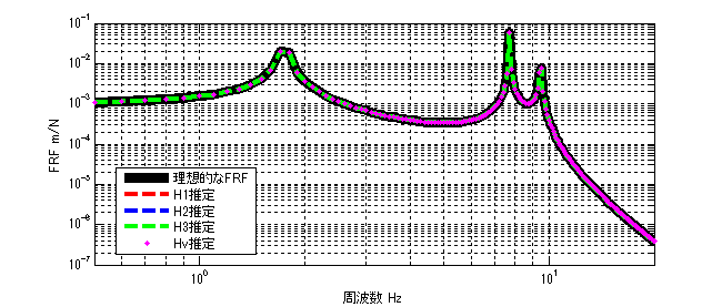
Figure 1: Error of 1%.
There is almost no difference. Since there is no use of consideration if there is no difference, I will give an error of 300% for now.
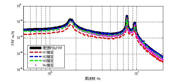
Figure 2: Error of 300%.
The order of the smallest difference from the ideal FRF is as follows
H2 estimation > H3 estimation > Hv estimation > H1 estimation
Case (2) where noise is included in the response (Execution file (2))
It is very common to get noise in the response.
In this case, for now, we gave an error of 3% based on the maximum amplitude X(ω). The result is shown below.
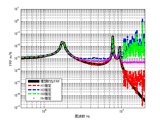
Figure 3: Error of 3%.
The order of the smallest difference from the ideal FRF is as follows
H1 estimation > Hv estimation > H3 estimation > H2 estimation
(3) Cases where noise is included in the input and response (executable file (3))
Although not realistic, the following figure shows the result when 300% noise is introduced into the input and 3% noise into the response.
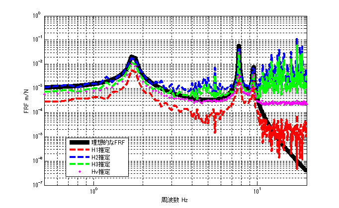
Figure 4: 300% error in input, 3% error in response
The order of the smallest difference from the ideal FRF is as follows
Hv estimate > H3 estimate > H2 estimate > H1 estimate
(We placed importance on the value at the resonant frequency and the absence of peaks at other frequencies)
Considering the normal experimental environment, I imagine that even if noise is mixed in, it is about 3% for the input and 5% for the response, and compare the results under these conditions.
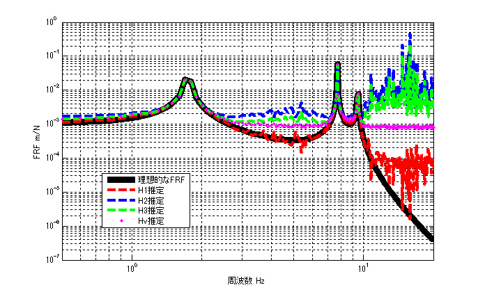
Figure 5: 3% error in input, 5% error in response
The order of the smallest difference from the ideal FRF is as follows
H1 estimate > Hv estimate > H3 estimate > H2 estimate
(We placed importance on the value at the resonant frequency and the absence of peaks at other frequencies)
In most FFT analyzers that can measure FRF, the default setting for FRF estimation method is “H1”. As shown in Fig. 3 and Fig. 5, “H1” estimation is considered to have the highest estimation accuracy in a normal measurement environment.
Under conditions other than those shown in Figures 3 and 5 (noisy environment), it is necessary to select an estimation method for each case.
MATLAB code
Executable file (1)
clear all
close all
% % % % 初期設定
freq=0.5:0.1:20;
m_vec=[1 1 1 1];
[M]=eval_Mmatrix(m_vec);
k_vec=[1 1 1 1]*10^3;
[K]=eval_Kmatrix(k_vec);
C=zeros(length(k_vec));
F=zeros(length(m_vec),length(freq));
F(1,:)=ones(1,length(freq));

% % % % 変位X(ノイズなし)
X=eval_direct_x_2ndedition(M,K,C,F,freq);
% % % % 理想的なFRF
FRF_ideal_x3_f1=X(3,:)./F(1,:);

N=100; %平均化回数 100回
res=zeros(N,length(freq));
ref=zeros(N,length(freq));
for ii1=1:N
    res(ii1,:)=X(3,:);
    ref(ii1,:)=F(1,:)+( rand(1,length(freq)) - 0.5 )*2*3; % Fを基準として±300%のノイズを加える
end

[h1] = FRF(ref,res,freq,'H1');
[h2] = FRF(ref,res,freq,'H2');
[h3] = FRF(ref,res,freq,'H3');
[hv] = FRF(ref,res,freq,'Hv');
[r2] = Coherence(ref,res,freq);

figure(1)
loglog(freq,abs(FRF_ideal_x3_f1),'k','linewidth',7)
hold on
loglog(freq,abs(h1),'r--','linewidth',3)
loglog(freq,abs(h2),'b--','linewidth',3)
loglog(freq,abs(h3),'g--','linewidth',3)
loglog(freq,abs(hv),'m.','linewidth',3)
hold off
grid on
legend('理想的なFRF','H1推定','H2推定','H3推定','Hv推定')
xlim([freq(1) freq(end)])
xlabel('周波数 Hz');ylabel('FRF m/N');

figure
semilogx(freq,r2,'k','linewidth',3)
xlabel('周波数 Hz');ylabel('Coherence');
grid on
ylim([0 1])
xlim([freq(1) freq(end)])
executable file (2)
clear all
close all
% % % % 初期設定
freq=0.5:0.1:20;
m_vec=[1 1 1 1];
[M]=eval_Mmatrix(m_vec);
k_vec=[1 1 1 1]*10^3;
[K]=eval_Kmatrix(k_vec);
C=zeros(length(k_vec));
F=zeros(length(m_vec),length(freq));
F(1,:)=ones(1,length(freq));

% % % % 変位X(ノイズなし)
X=eval_direct_x_2ndedition(M,K,C,F,freq);
% % % % 理想的なFRF
FRF_ideal_x3_f1=X(3,:)./F(1,:);

N=100; %平均化回数 100回
res=zeros(N,length(freq));
ref=zeros(N,length(freq));
for ii1=1:N
    res(ii1,:)=X(3,:)+( rand(1,length(freq)) - 0.5 )*max(abs(X(3,:)))*0.03; % 最大変位Xを基準として3%のノイズを加える
    ref(ii1,:)=F(1,:);
end

[h1] = FRF(ref,res,freq,'H1');
[h2] = FRF(ref,res,freq,'H2');
[h3] = FRF(ref,res,freq,'H3');
[hv] = FRF(ref,res,freq,'Hv');
[r2] = Coherence(ref,res,freq);

figure(1)
loglog(freq,abs(FRF_ideal_x3_f1),'k','linewidth',7)
hold on
loglog(freq,abs(h1),'r--','linewidth',3)
loglog(freq,abs(h2),'b--','linewidth',3)
loglog(freq,abs(h3),'g--','linewidth',3)
loglog(freq,abs(hv),'m.','linewidth',3)
hold off
grid on
legend('理想的なFRF','H1推定','H2推定','H3推定','Hv推定')
xlim([freq(1) freq(end)])
xlabel('周波数 Hz');ylabel('FRF m/N');

figure
semilogx(freq,r2,'k','linewidth',3)
xlabel('周波数 Hz');ylabel('Coherence');
grid on
ylim([0 1])
xlim([freq(1) freq(end)])
Executable file (3)
clear all
close all
% % % % 初期設定
freq=0.5:0.1:20;
m_vec=[1 1 1 1];
[M]=eval_Mmatrix(m_vec);
k_vec=[1 1 1 1]*10^3;
[K]=eval_Kmatrix(k_vec);
C=zeros(length(k_vec));
F=zeros(length(m_vec),length(freq));
F(1,:)=ones(1,length(freq));

% % % % 変位X(ノイズなし)
X=eval_direct_x_2ndedition(M,K,C,F,freq);
% % % % 理想的なFRF
FRF_ideal_x3_f1=X(3,:)./F(1,:);

N=100; %平均化回数 100回
res=zeros(N,length(freq));
ref=zeros(N,length(freq));
for ii1=1:N
    res(ii1,:)=X(3,:)+( rand(1,length(freq)) - 0.5 )*max(abs(X(3,:)))*0.05; % 最大変位Xを基準として5%のノイズを加える
    ref(ii1,:)=F(1,:)+( rand(1,length(freq)) - 0.5 )*2*0.03; % Fを基準として±3%のノイズを加える
end

[h1] = FRF(ref,res,freq,'H1');
[h2] = FRF(ref,res,freq,'H2');
[h3] = FRF(ref,res,freq,'H3');
[hv] = FRF(ref,res,freq,'Hv');
[r2] = Coherence(ref,res,freq);

figure(1)
loglog(freq,abs(FRF_ideal_x3_f1),'k','linewidth',7)
hold on
loglog(freq,abs(h1),'r--','linewidth',3)
loglog(freq,abs(h2),'b--','linewidth',3)
loglog(freq,abs(h3),'g--','linewidth',3)
loglog(freq,abs(hv),'m.','linewidth',3)
hold off
grid on
legend('理想的なFRF','H1推定','H2推定','H3推定','Hv推定')
xlim([freq(1) freq(end)])
xlabel('周波数 Hz');ylabel('FRF m/N');

figure
semilogx(freq,r2,'k','linewidth',3)
xlabel('周波数 Hz');ylabel('Coherence');
grid on
ylim([0 1])
xlim([freq(1) freq(end)])
function file
function [frf] = FRF(ref,res,freq,FRFtype)


switch FRFtype
    case 'H1'
        [frf] = H1(ref,res,freq);
    case 'H2'
        [frf] = H2(ref,res,freq);
    case 'H3'
        [frf] = H3(ref,res,freq);
    case 'Hv'
        [frf] = Hv(ref,res,freq);
end

end
function [h1] = H1(ref,res,freq)

% h1=zeros(1,freq);

[Wfx]=CrossSpectralDensity(ref,res,freq);
[Wff]=PowerSpectralDensity(ref,freq);

h1=mean(Wfx,1)./mean(Wff,1);

end
function [h2] = H2(ref,res,freq)

% h1=zeros(1,freq);

[Wxf]=CrossSpectralDensity(res,ref,freq);
[Wxx]=PowerSpectralDensity(res,freq);

h2=mean(Wxx,1)./mean(Wxf,1);

end
function [h3] = H3(ref,res,freq)

[h1] = H1(ref,res,freq);
[h2] = H2(ref,res,freq);

h3 = (h1 + h2)/2;
end
function [hv] = Hv(ref,res,freq)

[h1] = H1(ref,res,freq);
[h2] = H2(ref,res,freq);

hv = sqrt(h1).*sqrt(h2);
end
function [r2] = Coherence(ref,res,freq)

[h1] = H1(ref,res,freq);
[h2] = H2(ref,res,freq);

r2=h1./h2;

end
function [Wff]=PowerSpectralDensity(F,freq)

if size(F,1)==length(freq)
    F=F.';
end

Wff=conj(F).*F;
end
function [Wfx]=CrossSpectralDensity(F,X,freq)

if size(F,1)==length(freq)
    F=F.';
end
if size(X,1)==length(freq)
    X=X.';
end

Wfx=conj(F).*X;
end
function [K]=eval_Kmatrix(k_vec)
K=zeros(length(k_vec));
for ii1=1:length(k_vec)
    if ii1==1 K(ii1,ii1)=k_vec(ii1);
    else
        K(ii1-1:ii1,ii1-1:ii1)=K(ii1-1:ii1,ii1-1:ii1)+[1 -1;-1 1]*k_vec(ii1);
    end
end

end
function [M]=eval_Mmatrix(m_vec)
M=diag(m_vec);
end
function x=eval_direct_x_2ndedition(M,K,C,F,freq)
% % 2021.05.28 Fを修正
x=zeros(size(F,1),length(freq));
j=sqrt(-1);
for ii1=1:1:length(freq)
    w=2*pi*freq(ii1);
    x(:,ii1)=inv(K+j*w*C-w^2*M)*F(:,ii1);
end

end
コメント