H3 and Hv estimation of FRF

Introduction
H3 and Hv estimation of FRF
Theoretical expression
Validation in MATLAB
1. 関連

Introduction

There are several types of transfer functions (Frequency Response Function (FRF)): H1 estimation, H2 estimation, H3 estimation, and Hv estimation.
So far, we have introduced H1 and H2 estimation. This article describes H3 and Hv estimation.

If you want to see all my lessons in English, please see below.

TopPage 振動騒音研究所

MATLABとNVH(Noise, Vibration and Harshness)をこよなく愛する人生の先輩、それが私（MATLABパイセン）です。NVHを極めるにあたり、周辺の知識も網羅的に勉強することになり、その知識を共有すべく、本HPを運営しています。日本の製造業を応援すべく、機械エンジニアの「車輪の再開発」の防止と業務効率化の手助けをモットーに活動。専門である振動騒音工学や音響工学について、プログラムを示しながら解説。大学の授業よりもわかりやすく説明することを目指す。質問頂ければ、回答したいと思います。

We have explained that it is desirable to use H2 estimation when the input contains a noise component, and
H1 estimation should be used when the response contains a noise component.

H3 estimation or Hv estimation is the estimation method to use when the input & response contain noise.

Incidentally, I found the following explanation in “Introduction to Modal Analysis” written by Dr. Nagamatsu, which I have been reading with great interest.

The frequency response function when errors are mixed in both input and output is H3, which is defined approximately as follows, and Hv, which is strictly defined.

So H3 is approximate and Hv is exact.
Incidentally, “Introduction to Modal Analysis” does not present any theoretical formula for Hv estimation.

Theoretical expression

H3 estimation

The formula for H2 estimation in the textbook itself is very simple.

$$
H3(ω)= \frac{H1(ω)+H2(ω)}{2}
$$

Hv estimation

The formula for Hv estimation is below.
$$
Hv(ω)= \sqrt{H1(ω)} \sqrt{H2(ω)}
$$

Validation in MATLAB

Results

The results of the analysis are shown first. (100 times average)

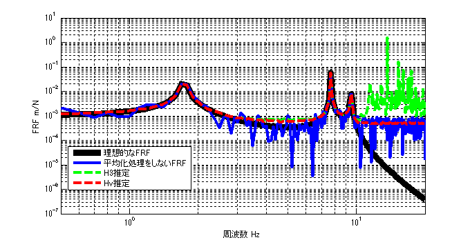
The ideal FRF with no noise component is shown by the black line.
The blue line represents the FRF without averaging and with noise components.
（The H3 estimation result (with averaging) is represented by the green dotted line, the Hv estimation result (with averaging) is represented by the red dotted line.
（The Hv estimation result (with averaging) is shown by the red dotted line.

What do you think?
Compared to the ideal FRF, both H3 and Hv estimation errors are large above 10 Hz, where the response is small.
As Dr. Nagamatsu said, Hv estimation seems to be more accurate than H3 estimation.

MATLAB code

Executable file

cleaclear all
close all
% % % % 初期設定
freq=0.5:0.1:20;
m_vec=[1 1 1 1];
[M]=eval_Mmatrix(m_vec);
k_vec=[1 1 1 1]*10^3;
[K]=eval_Kmatrix(k_vec);
C=zeros(length(k_vec));
F=zeros(length(m_vec),length(freq));
F(1,:)=ones(1,length(freq));

% % % % 変位X（ノイズなし）
X=eval_direct_x_2ndedition(M,K,C,F,freq);
% % % % 理想的なFRF
FRF_ideal_x3_f1=X(3,:)./F(1,:);

N=100; %平均化回数 100回
res=zeros(N,length(freq));
ref=zeros(N,length(freq));
for ii1=1:N
    res(ii1,:)=X(3,:)+( rand(1,length(freq)) - 0.5 )*max(abs(X(3,:)))*0.03; % 最大変位Xを基準として3%のノイズを加える
    ref(ii1,:)=F(1,:)+( rand(1,length(freq)) - 0.5 )*2*0.10; % Fを基準として±10%のノイズを加える
end

[h3] = H3(ref,res,freq);
[hv] = Hv(ref,res,freq);

figure(1)
loglog(freq,abs(FRF_ideal_x3_f1),'k','linewidth',7)
hold on
loglog(freq,abs(res(1,:)./ref(1,:)),'b','linewidth',3)
loglog(freq,abs(h3),'g--','linewidth',3)
loglog(freq,abs(hv),'r--','linewidth',3)
hold off
grid on
legend('理想的なFRF','平均化処理をしないFRF','H3推定','Hv推定')
xlim([freq(1) freq(end)])
xlabel('周波数 Hz');ylabel('FRF m/N');

function file

function [K]=eval_Kmatrix(k_vec)
K=zeros(length(k_vec)); 
for ii1=1:length(k_vec) 
    if ii1==1 K(ii1,ii1)=k_vec(ii1); 
    else 
        K(ii1-1:ii1,ii1-1:ii1)=K(ii1-1:ii1,ii1-1:ii1)+[1 -1;-1 1]*k_vec(ii1);
    end
end

end

function [M]=eval_Mmatrix(m_vec)
M=diag(m_vec);
end

function x=eval_direct_x_2ndedition(M,K,C,F,freq)
% % 2021.05.28 Fを修正 
x=zeros(size(F,1),length(freq));
j=sqrt(-1);
for ii1=1:1:length(freq)
    w=2*pi*freq(ii1);
    x(:,ii1)=inv(K+j*w*C-w^2*M)*F(:,ii1);
end

end

function [Wff]=PowerSpectralDensity(F,freq)

if size(F,1)==length(freq)
    F=F.';
end

Wff=conj(F).*F;


end

function [Wfx]=CrossSpectralDensity(F,X,freq)

if size(F,1)==length(freq)
    F=F.';
end
if size(X,1)==length(freq)
    X=X.';
end



Wfx=conj(F).*X;


end

function [h1] = H1(ref,res,freq)

% h1=zeros(1,freq);

[Wfx]=CrossSpectralDensity(ref,res,freq);
[Wff]=PowerSpectralDensity(ref,freq);

h1=mean(Wfx,1)./mean(Wff,1);

end

function [h2] = H2(ref,res,freq)

% h1=zeros(1,freq);

[Wxf]=CrossSpectralDensity(res,ref,freq);
[Wxx]=PowerSpectralDensity(res,freq);

h2=mean(Wxx,1)./mean(Wxf,1);

end

function [h3] = H3(ref,res,freq)

[h1] = H1(ref,res,freq);
[h2] = H2(ref,res,freq);

h3 = (h1 + h2)/2;
end

function [hv] = Hv(ref,res,freq)

[h1] = H1(ref,res,freq);
[h2] = H2(ref,res,freq);

hv = sqrt(h1).*sqrt(h2);
end

Introduction