Introduction
The “fft” function in MATLAB does not match the frequency analysis results (spectrum) of the vibration and noise. This article describes a frequency analysis method that is consistent with commercial software like B&K or LMS.
If you want to see all my lessons in English, please see below.

Amplitude and RMS
There is a time signal with amplitude A as shown in the figure below. If you want to obtain the spectrum by fft, it is necessary to clarify whether you want to obtain the amplitude A or the RMS value of the amplitude. Generally, vibration and noise are evaluated by “RMS value”.

Figure 1 Signal
Here, the amplitude A is called “peak,” and the RMS value is called “RMS”.
Then, we can summarize the results as follows.
Table 1 Comparison table
| peak | RMS | |
| Spectrum | A | A/√2 |
| Autopower | A^2 | A^2/2 |
| PSD | A^2/df | A^2/2/df |
Correction coefficients for window functions
Next, we will explain how to correct for the use of the window function. The correction coefficients depends on the type of window function.
Table 2 Window function correction coefficients
| rectangular | hanning | hamming | blackman | |
| Spectrum | 1 | 1/0.5 | 1/0.54 | 1/0.42 |
| Autopower (for frequency response) |
1^2 | (1/0.5 )^2 | ( 1/0.54 )^2 | ( 1/0.42 )^2 |
| Auto- power (for bandwidth calculation) |
1 | 8/3 | (50^2*2/(27^2*2+23^2) | (25^2*2^3)/(21^2*2+25^2+2^2) |
| PSD | 1 | 8/3 | (50^2*2/(27^2*2+23^2) | (25^2*2^3)/(21^2*2+25^2+2^2) |
MATLAB code
Confirmation of function file operation
The following figures show the results of checking the operation of function files.
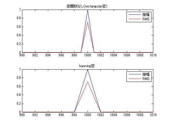
Figure 2 Spectrum
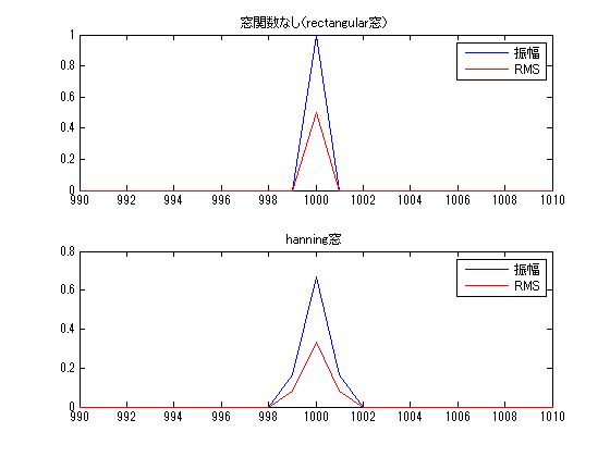
Figure 3 Auto- power
In the Autopower results in Figure 3, the amplitude values differ between the rectangular and Hanning windows, but the Hanning window has components (amplitude values) at 999Hz and 1001Hz. Adding the amplitude values between 999Hz and 1001Hz in the Hanning window, the amplitude values in the rectangular window match the amplitude values in the rectangular window. This means that the O.A. values and octave analysis results are corrected to match.
Execution code (for checking the operation of function files)
clear all;clc;close all

fs=1024*4;
t=linspace(0,1,fs+1);
sig=sin(2*pi*1000*t);
[freq,fft_coe,peak_fftdata,RMS_fftdata]=fft4Spectrum(sig,fs,fs,'rectangular');
[freq,fft_coe,peak_power,RMS_power]=fft4Power(sig,fs,fs,'rectangular');
figure(1)
subplot(211)
plot(freq,abs(peak_fftdata))
hold on
plot(freq,abs(RMS_fftdata),'r')
legend('振幅','RMS')
xlim([990 1010])
title('窓関数なし(rectangular窓)')

figure(2)
subplot(211)
plot(freq,abs(peak_power))
hold on
plot(freq,abs(RMS_power),'r')
legend('振幅','RMS')
xlim([990 1010])
title('窓関数なし(rectangular窓)')


[freq,fft_coe,peak_fftdata,RMS_fftdata]=fft4Spectrum(sig,fs,fs,'hanning');
[freq,fft_coe,peak_power,RMS_power]=fft4Power(sig,fs,fs,'hanning');
figure(1)
subplot(212)
plot(freq,abs(peak_fftdata))
hold on
plot(freq,abs(RMS_fftdata),'r')
legend('振幅','RMS')
xlim([990 1010])
title('hanning窓')

figure(2)
subplot(212)
plot(freq,abs(peak_power))
hold on
plot(freq,abs(RMS_power),'r')
legend('振幅','RMS')
xlim([990 1010])
title('hanning窓')
function file
(fft for spectrum)
function [freq,fft_coe,peak_fftdata,RMS_fftdata]=fft4Spectrum(sig,fs,N,window)
% % % % input
% sig   : 時刻歴信号
% N     : fftのデータ数(Line数)
% fs    : サンプリング周波数
% window: 窓関数名(レクタンギュラ窓、ハニング窓、ハミング窓、ブラックマン窓が使用可能)
%
% % % % output
% freq    :周波数
% fft_coe :窓関数の補正係数
% peak_fftdata :時間信号の振幅を求めたい場合に使用
% RMS_fftdata  :実効値のfft結果(通常、振動騒音ではこれを使う)
%
% ★注意
% -------パワーを計算したい場合は下記計算をすること-------
% peak_fftdata.^2/fft_coe(1)^2*fft_coe(2)
% RMS_fftdata.^2/fft_coe(1)^2*fft_coe(2)

% size(sig)は(1,length(sig))となるようにしたいので、ここでチェック
if size(sig,1)==length(sig)
    sig=sig.';
end
[win,fft_coe]=get_window(length(sig),window);
fftdata=fft(sig.*win,N)/N;

freq=linspace(0,fs/2,floor(N/2)+1);
% % % peak(時間信号の振幅を求めたいとき)
peak_fftdata=fftdata(1:floor(N/2)+1)*2*fft_coe(1); %負の周波数分の補正

% % % RMS(実効値)
RMS_fftdata=peak_fftdata/sqrt(2);

end


function [win,fft_coe]=get_window(N,window)
t=linspace(0,1,N);
switch window
    case 'rectangular'
        win = ones(1,N);
        fft_coe=[1 1];
    case 'hanning'
        win = 0.5*ones(1,N) - 0.5*cos(2.0*pi*t);
        fft_coe=[2 8/3];
    case 'hamming'
        win = 0.54*ones(1,N) - 0.46*cos(2.0*pi*t);
        fft_coe=[1/0.54 1/( (27^2*2+23^2)/(50^2*2) )];
    case 'blackman'
        win = 0.42*ones(1,N) - 0.5*cos(2.0*pi*t) + 0.08*cos(4.0*pi*t);
        fft_coe=[1/0.42 1/( (21^2*2+25^2+2^2)/(25^2*2^3) )];
end

end
(fft for power)
This is used to calculate the power of a band, such as O.A. value or octave analysis.
function [freq,fft_coe,peak_fftdata,RMS_fftdata]=fft4Power(sig,fs,N,window)
% % % % input
% sig   : 時刻歴信号
% N     : fftのデータ数(Line数)
% fs    : サンプリング周波数
% window: 窓関数名(レクタンギュラ窓、ハニング窓、ハミング窓、ブラックマン窓が使用可能)
%
% % % % output
% freq    :周波数
% fft_coe :窓関数の補正係数
% peak_fftdata :時間信号の振幅を求めたい場合に使用
% RMS_fftdata  :実効値のfft結果(通常、振動騒音ではこれを使う)
%

% size(sig)は(1,length(sig))となるようにしたいので、ここでチェック
if size(sig,1)==length(sig)
    sig=sig.';
end
[win,fft_coe]=get_window(length(sig),window);
fftdata=fft(sig.*win,N)/N;

freq=linspace(0,fs/2,floor(N/2)+1);
fftdata=fftdata(1:floor(N/2)+1)*2; %負の周波数分の補正
% % % peak(時間信号の振幅を求めたいとき)
peak_fftdata=fftdata.^2*fft_coe(2);

% % % RMS(実効値)
RMS_fftdata=peak_fftdata/2;

end


function [win,fft_coe]=get_window(N,window)
t=linspace(0,1,N);
switch window
    case 'rectangular'
        win = ones(1,N);
        fft_coe=[1 1];
    case 'hanning'
        win = 0.5*ones(1,N) - 0.5*cos(2.0*pi*t);
        fft_coe=[2 8/3];
    case 'hamming'
        win = 0.54*ones(1,N) - 0.46*cos(2.0*pi*t);
        fft_coe=[1/0.54 1/( (27^2*2+23^2)/(50^2*2) )];
    case 'blackman'
        win = 0.42*ones(1,N) - 0.5*cos(2.0*pi*t) + 0.08*cos(4.0*pi*t);
        fft_coe=[1/0.42 1/( (21^2*2+25^2+2^2)/(25^2*2^3) )];
end

end
Extra (Derivation of Correction Factors for Window Functions)
The amplitude is reduced by the window function. For auto power, the amount of reduction can be obtained by finding the integral of the square of the window function. Since this 1/reduction is the correction factor, I calculated the integral. (Sorry if this is wrong)


コメント