Introduction
When identifying resonant frequencies and vibration modes, we look at the FRF peaks and think “I wonder if this is the resonant frequency”.
However, it is not always the case that (peak FRF frequency) = (resonant frequency).
As those who have experienced hammering or excitation tests, the lower-order FRF peak value is easy to determine as the resonance frequency, but the higher-order FRF peak value is not.
The higher-order FRF peak values are densely concentrated in a narrow band, making it difficult to determine whether they are resonance frequencies, just peak values, or noise.
It is also impossible to determine the overlapping roots (when two resonance frequencies exist at the same frequency).
This article explains how to identify the resonance frequency using the mode indicator function.
The following link is a summary to a description of vibration theory in English, if you are interested.

I’ve also developed my own curve fitting software.
If you’re interested, feel free to download it from the link below and give it a try.
👉 Free Download
Modal Indicator Functions
Do you know Modal Indicator Functions(MIFs)?
There are several types of modal indicator functions: CMIF, MMIF, and RMIF.
Here, CMIF (Complex Modal Indicator Functions) are introduced.
Ewin’s book “Modal Testing” provides the explanation of modal indicator functions.
CMIF(Complex Modal Indicator Functions)
The following are the theoretical equations for CMIF. The theoretical equation is based on the following reference.
CMIF is expressed as the singular value decomposition of the transfer function matrix H(ω), as shown in the equation below.
$$
H(ω)=U∑V
$$
$$
CIMF(ω)=∑^{T}∑
$$
Validation in MATLAB
Verification with executable file ①.
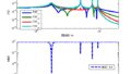
The CMIF results for 1-point excitation and 4-point response are shown in the figure below. Note that in the case of 1-point excitation, only the first-order CMIF can be obtained. (Only the result of the maximum singular value can be obtained.)
From the figure, it can be seen that the resonance frequency and the peak value of CMIF coincide.
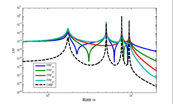 Figure 1 Result of executable file ①
As it is, we can’t see much good in CMIF; the good thing about CMIF is the identification of the heavy roots.
Verification with executable file ②
To take it a step further, modify the executable ① slightly to obtain the CMIF for a 2-point excitation and a 4-point response.
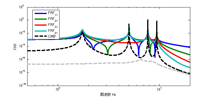
Figure 2 Result of Run File ②
In the case of two-point excitation, the first-order and second-order CMIFs are obtained (black dotted line for first-order, gray dotted line for second-order). (First-order is black dotted line, second-order is gray dotted line)
Verification with executable file ③
Now let’s examine the case with heavy roots: we have adjusted the mass and spring constant so that there are two resonance frequencies near 5 Hz. Under these conditions, we obtain the CMIF for a two-point excitation and four-point response.
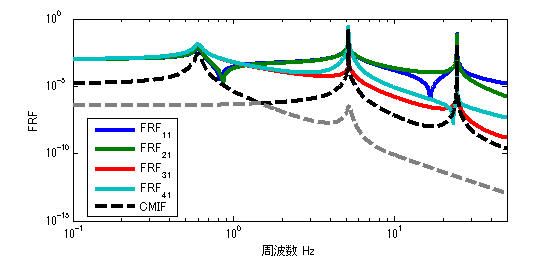 Figure 3 Result of Run File ③
As in the case of run file ②, the first-order and second-order CMIFs are obtained in the case of two-point excitation. (First-order is black dotted line, second-order is gray dotted line)
Now, looking at the FRF results alone, it looks like the resonant frequency is only 3.
But what if we check the CMIF?
We can see that there are three resonant frequencies in the first-order CMIF.
The second-order CMIF also has a peak near 5 Hz, indicating that there is another resonant frequency near 5 Hz.
Summary of CMIF features and benefits
- CMIF peaks appear at resonant frequencies
- Even if there are multiple resonant frequencies in a narrow band, the second- and third-order (higher-order) CMIF results can be used to determine the overlapping roots.
Perhaps there is no other site that explains the mode-directed functions so carefully, so I hope this will be of some help.
MATLAB code
Executable file ①.
clear all
close all
% % % % 初期設定
freq=0.5:0.01:20;
m_vec=[1 1 1 1];
[M]=eval_Mmatrix(m_vec);
k_vec=[1 1 1 1]*10^3;
[K]=eval_Kmatrix(k_vec);
C=ones(length(k_vec))*0.1;
F1=zeros(length(m_vec),length(freq));
F1(1,:)=ones(1,length(freq));
F2=zeros(length(m_vec),length(freq));
F2(2,:)=ones(1,length(freq));
% % % % 変位X(ノイズなし)
X1=eval_direct_x_2ndedition(M,K,C,F1,freq);
X2=eval_direct_x_2ndedition(M,K,C,F2,freq);
% % % % 理想的なFRF
FRF_x4_f1=X1(4,:)./F1(1,:);
FRF_x3_f1=X1(3,:)./F1(1,:);
FRF_x2_f1=X1(2,:)./F1(1,:);
FRF_x1_f1=X1(1,:)./F1(1,:);

FRF_x4_f2=X2(4,:)./F2(2,:);
FRF_x3_f2=X2(3,:)./F2(2,:);
FRF_x2_f2=X2(2,:)./F2(2,:);
FRF_x1_f2=X2(1,:)./F2(2,:);


inputN=1;
CMIF_vector=zeros(inputN,length(freq));

for ii1=1:length(freq)
    H=[ FRF_x1_f1(ii1) %FRF_x1_f2(ii1)
        FRF_x2_f1(ii1) %FRF_x2_f2(ii1)
        FRF_x3_f1(ii1) %FRF_x3_f2(ii1)
        FRF_x4_f1(ii1) %FRF_x4_f2(ii1)
        ];
    [U,S,V] = svd(H);
    CMIF_vector(:,ii1)=diag(S.'*S);
end

figure
loglog(freq,abs([FRF_x1_f1;FRF_x2_f1;FRF_x3_f1;FRF_x4_f1]),'linewidth',3)
hold on
loglog(freq,CMIF_vector,'k--','linewidth',3)
xlim([freq(1) freq(end)])
xlabel('周波数 Hz');ylabel('FRF');
legend('FRF_1_1','FRF_2_1','FRF_3_1','FRF_4_1','CMIF')
Executable file ②
clear all
close all
% % % % 初期設定
freq=0.5:0.01:20;
m_vec=[1 1 1 1];
[M]=eval_Mmatrix(m_vec);
k_vec=[1 1 1 1]*10^3;
[K]=eval_Kmatrix(k_vec);
C=ones(length(k_vec))*0.1;
F1=zeros(length(m_vec),length(freq));
F1(1,:)=ones(1,length(freq));
F2=zeros(length(m_vec),length(freq));
F2(2,:)=ones(1,length(freq));
% % % % 変位X(ノイズなし)
X1=eval_direct_x_2ndedition(M,K,C,F1,freq);
X2=eval_direct_x_2ndedition(M,K,C,F2,freq);
% % % % 理想的なFRF
FRF_x4_f1=X1(4,:)./F1(1,:);
FRF_x3_f1=X1(3,:)./F1(1,:);
FRF_x2_f1=X1(2,:)./F1(1,:);
FRF_x1_f1=X1(1,:)./F1(1,:);

FRF_x4_f2=X2(4,:)./F2(2,:);
FRF_x3_f2=X2(3,:)./F2(2,:);
FRF_x2_f2=X2(2,:)./F2(2,:);
FRF_x1_f2=X2(1,:)./F2(2,:);


inputN=2;
CMIF_vector=zeros(inputN,length(freq));

for ii1=1:length(freq)
    H=[ FRF_x1_f1(ii1) FRF_x1_f2(ii1)
        FRF_x2_f1(ii1) FRF_x2_f2(ii1)
        FRF_x3_f1(ii1) FRF_x3_f2(ii1)
        FRF_x4_f1(ii1) FRF_x4_f2(ii1)
        ];
    [U,S,V] = svd(H);
    CMIF_vector(:,ii1)=diag(S.'*S);
end

figure
loglog(freq,abs([FRF_x1_f1;FRF_x2_f1;FRF_x3_f1;FRF_x4_f1]),'linewidth',3)
hold on
loglog(freq,CMIF_vector,'k--','linewidth',3)
xlim([freq(1) freq(end)])
xlabel('周波数 Hz');ylabel('FRF');
legend('FRF_1_1','FRF_2_1','FRF_3_1','FRF_4_1','CMIF')
Executable file ③
clear all
close all
% % % % 初期設定
freq=0.1:0.01:50;
m_vec=[0.80 0.98 30 0.95];
[M]=eval_Mmatrix(m_vec);
k_vec=[1 10 0.90 1]*10^3;
[K]=eval_Kmatrix(k_vec);
 [V,D] = eig(K,M);
fn=sqrt(diag(D))/(2*pi);

C=ones(length(k_vec))*1;
F1=zeros(length(m_vec),length(freq));
F1(1,:)=ones(1,length(freq));
F2=zeros(length(m_vec),length(freq));
F2(2,:)=ones(1,length(freq));
F3=zeros(length(m_vec),length(freq));
F3(3,:)=ones(1,length(freq));
% % % % 変位X(ノイズなし)
X1=eval_direct_x_2ndedition(M,K,C,F1,freq);
X2=eval_direct_x_2ndedition(M,K,C,F2,freq);
X3=eval_direct_x_2ndedition(M,K,C,F3,freq);
% % % % 理想的なFRF
FRF_x4_f1=X1(4,:)./F1(1,:);
FRF_x3_f1=X1(3,:)./F1(1,:);
FRF_x2_f1=X1(2,:)./F1(1,:);
FRF_x1_f1=X1(1,:)./F1(1,:);

FRF_x4_f2=X2(4,:)./F2(2,:);
FRF_x3_f2=X2(3,:)./F2(2,:);
FRF_x2_f2=X2(2,:)./F2(2,:);
FRF_x1_f2=X2(1,:)./F2(2,:);

FRF_x4_f3=X3(4,:)./F3(3,:);
FRF_x3_f3=X3(3,:)./F3(3,:);
FRF_x2_f3=X3(2,:)./F3(3,:);
FRF_x1_f3=X3(1,:)./F3(3,:);


inputN=2;
CMIF_vector=zeros(inputN,length(freq));

for ii1=1:length(freq)
    H=[ FRF_x1_f1(ii1) FRF_x1_f3(ii1)
        FRF_x2_f1(ii1) FRF_x2_f3(ii1)
        FRF_x3_f1(ii1) FRF_x3_f3(ii1)
        FRF_x4_f1(ii1) FRF_x4_f3(ii1)
        ];
    [U,S,V] = svd(H);
    CMIF_vector(:,ii1)=diag(S.'*S);
end

figure
loglog(freq,abs([FRF_x1_f1;FRF_x2_f1;FRF_x3_f1;FRF_x4_f1]),'linewidth',3)
hold on
loglog(freq,CMIF_vector,'k--','linewidth',3)
xlim([freq(1) freq(end)])
xlabel('周波数 Hz');ylabel('FRF');
legend('FRF_1_1','FRF_2_1','FRF_3_1','FRF_4_1','CMIF')
function file
function [K]=eval_Kmatrix(k_vec)
K=zeros(length(k_vec));
for ii1=1:length(k_vec)
    if ii1==1 K(ii1,ii1)=k_vec(ii1);
    else
        K(ii1-1:ii1,ii1-1:ii1)=K(ii1-1:ii1,ii1-1:ii1)+[1 -1;-1 1]*k_vec(ii1);
    end
end

end
function [M]=eval_Mmatrix(m_vec)
M=diag(m_vec);
end
function x=eval_direct_x_2ndedition(M,K,C,F,freq)
% % 2021.05.28 Fを修正
x=zeros(size(F,1),length(freq));
j=sqrt(-1);
for ii1=1:1:length(freq)
    w=2*pi*freq(ii1);
    x(:,ii1)=inv(K+j*w*C-w^2*M)*F(:,ii1);
end

end
コメント