
Introduction
In recent years, the trend at overseas universities is not to delve deeply into purely vibration or mechanical engineering, but rather research and words such as digital twin, condition monitoring, 1DCAE, MBD, and metamaterials are becoming more prominent. These fields require cross-fertilization of disciplines that were considered as other fields a long time ago, such as vibration engineering + control engineering + IoT + systems. Therefore, Japanese universities, where laboratories are often run by a single professor, have not been able to conduct cutting-edge research in these fields. Especially in the field of vibration, there has been no excellent research on the above-mentioned research themes.
The “Kalman filter” introduced here is a method for estimating state variables, and when state “variables” = “vibration”, vibration estimation becomes possible. Therefore, it is applied in fields such as digital twin and condition monitoring.
The Kalman filter itself is very widely known in control engineering and is a theory that seems to have been worked out quite well in control engineering. However, in control engineering, it is applied to models with a few degrees of freedom and could not handle frequency bands like those handled in vibration engineering, but overseas universities are aiming to apply it to frequency bands like those handled in vibration engineering.
The above trends are not very familiar to Japanese people who make their living in vibration engineering, are they? In the first place, you may not have caught the trend.
Since there is not much good literature from Japanese universities, this article will refer to the paper in this link.
In this article, we would like to explain how to solve a state-space model in a continuous-time system as a preliminary step to learning the Kalman filter. If you have not read the previous article, please also refer to the following.

If you want to see all my lessons in English, please see below.

State space model (spring-mass-damper model with N degrees of freedom)
Since this is a duplicate of the previous article, I will only briefly describe the review part. The equation of motion for N degrees of freedom as shown in Figure 1 is equation (1). Please refer to the previous article for an explanation of the detailed character equation.

Figure 1: Springmass model (N degrees of freedom)
$$
[M][ddot{y} (t)] + [C][dot{y} (t)] + [K][y(t)]=[u(t)] \tag{1}
$$
From equation (1), the equation of state is now equation (3), and the output equation is now equation (4).
$$
\left( \begin{array}{c}
[ \dot{x_1}] \\
[ \dot{x_2}]
\end{array} \right) =
\left( \begin{array}{cc}
[0] & [I] \\
-[M]^{-1}[K] & -[M]^{-1}[C]
\end{array} \right)
\left( \begin{array}{c}
[x_1] \\
[x_2] [u]
\end{array} \right) +
\left( \begin{array}{c}
[0] \\
[M]^{-1}
\end{array} \right) \tag{3}
$$
$$
[y]=
\left( \begin{array}{cc}
[I] & [0]
\end{array} \right)
\left( \begin{array}{c}
[x_1] \\
[x_2]
\end{array} \right) \tag{4}
$$
Generalizing, you have equation (5).
\begin{eqnarray}
\left\{
\begin{array}{l}
[\dot{x} (t)] = [A][x(t)]+[B][u(t)] \\
[y(t)] = [C] [x(t)]
\end{array}
\right.
\tag{5}
\end{eqnarray}
Since the state-space model (state and output equations) is a continuous-time system, it must be discretized in order to apply the Kalman filter. However, even if we talk about discretization, you will not understand discretization unless you know how to solve continuous-time systems, so I will explain how to solve continuous-time systems.
In MATLAB, I would like to compare the “ode45” method for solving differential equations for continuous-time systems with the Eulerian and fourth-order Runge-Kutta methods.
Euler method
The Euler method is an approximate calculation of the state x(t+Δt) after Δt as follows.
$$
[x(t+Δt)]=[x(t)]+([A][x(t)]+[B][u(t)])Δt \tag{8}
$$
Runge-Kutta Method
The Runge-Kutta method is an approximate calculation of the state x(t+Δt) after Δt by expanding the Taylor series around t. A commonly used form of the method is to consider terms up to the fourth order of Δt and neglect terms after the fifth order.
$$
[x(t+Δt)]=[x(t)]+frac{d_1+2d_2+2d_3+d_4}{6} \tag{9}
$$
However,
$$
dot{x}(t)=f(x(t))
$$
\begin{eqnarray}
\left\{
\begin{array}{l}
d_1=f(x(t))Δt \\
d_2=f(x(t)+d_1/2)Δt \\
d_3=f(x(t)+d_2/2)Δt \\
d_4=f(x(t)+d_3)Δt
\end{array}
\right. \tag{10}
\end{eqnarray}
State space model solved in MATLAB (N-degree-of-freedom model)
Now let’s compare with “ode45” using the previous example.
- Degrees of freedom N=10
- k=10^5
- c=1
- m=1
- Sampling frequency fs=400 (dt=1/fs)
- Initial value of x: 1 for displacement of m1, 0 for displacement of m2 to m10
- State variable to be determined: acceleration
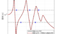
Displacements and velocities for all degrees of freedom are obtained, but only the results for the displacement of m10 are presented here.

Figure 2 Comparison of solution methods (Green line: Euler method, Red line: Runge-Kutta method)
If “ode45” in MATLAB is correct, then I see that the 4th order Runge-Kutta method is analyzing the data with a good degree of accuracy there. However, the Euler method does not match the amplitudes at all, and is not likely to be useful in an analysis such as this model.
This article simply explains how to solve the state-space model as a continuous-time system. The program we used is attached below.
MATLAB code
Executable file
clear all;clc;close all

m_vec=ones(1,10);
k_vec=ones(1,10)*10^5;
[M]=eval_Mmatrix(m_vec); %Mass Matrix
[K]=eval_Kmatrix(k_vec); %Stiffness Matrix
C=K*10^-5;

[V,D]=eig(K,M); %eigenvalue D、eigen vector V
wn=sqrt(diag(D)); %Eig Anguler Freq.
fn=wn/(2*pi); %Eig Freq.


% % Equation of state (continuous time system)
% % dx/dt =Ac x(t) + Bc p(t)
Ac=[zeros(size(M)) eye(size(M))
    -inv(M)*K -inv(M)*C];
Bc=[zeros(size(M))
    -inv(M)];

Cc=[-inv(M)*K -inv(M)*C];

x0 = zeros(size(M,1)*2,1);
x0(1) =1;
t0 = 0;
dt=1/400;
tf = 10;
time=t0:dt:tf;

% % % % % % % % % % % MATLAB ode45
[T,Y] = ode45(@state_equation, time, x0);
figure
% subplot(211)
plot(T,Y(:,10),'k','linewidth',2)
xlabel('Time [s]')
ylabel('Displacement [m]')
% subplot(212)
% y_k=Cc*Y.';
% plot(T,y_k(10,:))
% xlabel('Time [s]')
% ylabel('Acc. [m/s^2]')


% % % % % % % % % % % Euler
time=T.'; dt=T(2)-T(1);
p=zeros(size(M,1),1);
x_Euler_Method=zeros(length(M)*2,length(time));
x=x0;
for ii1=1:1:length(time)
    x_Euler_Method(:,ii1)=x;
    dx=Ac*x+Bc*p;
    x = x + dx*dt;
end
% subplot(211)
hold on
plot(time,x_Euler_Method(10,:),'--g','linewidth',1)
% % % % % % % % % % %

% % % % % % % % % % % Runge-Kutta
p=zeros(size(M,1),1);
x_RungeKutta_Method=zeros(length(M)*2,length(time));
x=x0;
d=zeros(length(M)*2,4);
for ii1=1:1:length(time)
    x_RungeKutta_Method(:,ii1)=x;
% % % % % % % d1
        xt=x;
        f = Ac*x + Bc*p;
        d(:,1) = f*dt;
% % % % % % % d2
        x = xt + d(:,1)*0.5;
        f = Ac*x + Bc*p;
        d(:,2) = f*dt;
% % % % % % % d3
        x = xt + d(:,2)*0.5;
        f = Ac*x + Bc*p;
        d(:,3) = f*dt;
% % % % % % % d3
        x = xt + d(:,3);
        f = Ac*x + Bc*p;
        d(:,4) = f*dt;
    x = xt + (d(:,1) + d(:,2)*2 +d(:,3)*2 +d(:,4) )/6;
end
% subplot(211)
hold on
plot(time,x_RungeKutta_Method(10,:),'-r','linewidth',2)
ylim([-1 1])
xlim([0 0.3])
legend('ode45','Euler','Runge-Kutta')
function file
function [M]=eval_Mmatrix(m_vec)

M=diag(m_vec);

end
function [K]=eval_Kmatrix(k_vec)

K=zeros(length(k_vec));
for ii1=1:length(k_vec)
    if ii1==1
        K(ii1,ii1)=k_vec(ii1);
    else
        K(ii1-1:ii1,ii1-1:ii1)=K(ii1-1:ii1,ii1-1:ii1)+[1 -1;-1 1]*k_vec(ii1);
    end
end

end
function dx=state_equation(t,x)


m_vec=ones(1,10);
k_vec=ones(1,10)*10^5;
[M]=eval_Mmatrix(m_vec); %Mass Matrix
[K]=eval_Kmatrix(k_vec); %Stiffness Matrix
C=K*10^-5;


% % Equation of state (continuous time system)
% % dx/dt =Ac x(t) + Bc p(t)
Ac=[zeros(size(M)) eye(size(M))
    -inv(M)*K -inv(M)*C];
Bc=[zeros(size(M))
    -inv(M)];

% Cc=[-Sa*inv(M)*K -Sa*inv(M)*C];
% Dc=Sa*inv(M);
p=zeros(size(M,1),1);
% size(p)
% size(Bc)
% size(Bc*p)
%
% size(Ac)
% size(Ac*x)
dx=Ac*x+Bc*p;
end
コメント