
Introduction
In recent years, the trend at overseas universities is not to delve deeply into purely vibration or mechanical engineering, but rather research and words such as digital twin, condition monitoring, 1DCAE, MBD, and metamaterials are becoming more prominent. These fields require cross-fertilization of disciplines that were considered as other fields a long time ago, such as vibration engineering + control engineering + IoT + systems. Therefore, Japanese universities, where laboratories are often run by a single professor, have not been able to conduct cutting-edge research in these fields. Especially in the field of vibration, there has been no excellent research on the above-mentioned research themes.
The “Kalman filter” introduced here is a method for estimating state variables, and when state “variables” = “vibration”, vibration estimation becomes possible. Therefore, it is applied in fields such as digital twin and condition monitoring.
The Kalman filter itself is very widely known in control engineering and is a theory that seems to have been worked out quite well in control engineering. However, in control engineering, it is applied to models with a few degrees of freedom and could not handle frequency bands like those handled in vibration engineering, but overseas universities are aiming to apply it to frequency bands like those handled in vibration engineering.
The above trends are not very familiar to Japanese people who make their living in vibration engineering, are they? In the first place, you may not have caught the trend.
Since there is not much good literature from Japanese universities, this article will refer to the paper in this link.
In this article, we would like to explain how to solve the state-space model as a preliminary step to learning the Kalman filter.
If you want to see all my lessons in English, please see below.

State space model (spring-mass-damper model with N degrees of freedom)
Those who study and research mainly vibration engineering and experimental modal analysis may not be familiar with “state-space models,” so here is a brief explanation. A state-space model is a type of model used in time series analysis, and is represented by a state equation and an output equation. In this article, we will develop the equations using the N-degree-of-freedom spring-mass-damper model shown in Figure 1.

Figure 1: Springmass model (N degrees of freedom)
The equations of motion for the spring-mass-damper model shown in Figure 1 can be expressed as in Equation (1) with input u(t) and displacement y(t). Note that [] denotes matrices and vectors.
$$
[M][ddot{y} (t)] + [C][dot{y} (t)] + [K][y(t)]=[u(t)] \tag{1}
$$
The equation of motion in equation (1) is divided into two variables, displacement x1 and velocity x2, as in equation (2). (Only here, time (t) is omitted, but this is of no particular significance.)
\begin{eqnarray}
\left\{
\begin{array}{l}
[x_1(t)] = [y(t)] \\
[x_2(t)] = [ \dot{y} (t)]
\end{array}
\right.
\tag{2}
\end{eqnarray}
Using equation (2), the equation of state can be expressed as in equation (3).
$$
\left( \begin{array}{c}
[ \dot{x_1}] \\
[ \dot{x_2}]
\end{array} \right) =
\left( \begin{array}{cc}
[0] & [I] \\
-[M]^{-1}[K] & -[M]^{-1}[C]
\end{array} \right)
\left( \begin{array}{c}
[x_1] \\
[x_2] [u]
\end{array} \right) +
\left( \begin{array}{c}
[0] \\
[M]^{-1}
\end{array} \right) \tag{3}
$$
The output equation is equation (4). Remember that the output equation happens to be the displacement x1, although we often deal with equation (4) in vibration-related output equations. (In future problems, you will be dealing with output equations that output only m1 acceleration, for example.)
$$
[y]=
\left( \begin{array}{cc}
[I] & [0]
\end{array} \right)
\left( \begin{array}{c}
[x_1] \\
[x_2]
\end{array} \right) \tag{4}
$$
Equations (3) and (4) can be summarized as in Equation (5). Here, we can organize equation (5) in text form as follows.
- State equation: relationship between input u and state vector x
- Output equation: relationship between state vector x and output y
In other words, the output equation can be in any equation form that can be obtained from the state vector, and you can see that “Equation (4) is not the only output equation for the equation of motion.
\begin{eqnarray}
\left\{
\begin{array}{l}
[\dot{x} (t)] = [A][x(t)]+[B][u(t)] \\
[y(t)] = [C] [x(t)]
\end{array}
\right.
\tag{5}
\end{eqnarray}
So how would you make the output equation an acceleration instead of a displacement?
The answer is equation (6).
$$
[y]=
\left( \begin{array}{cc}
-[M]^{-1}[K] & -[M]^{-1}[C]
\end{array} \right)
\left( \begin{array}{c}
[x_1] \\
[x_2]
\end{array} \right) \tag{6}
$$
In fact, the state-space model (state and output equations) is a continuous-time system and must be discretized so that it can be solved numerically, but MATLAB has a function called “ode45” that solves differential equations for continuous-time systems, so this is the end of today’s theoretical explanation.
State space model solved in MATLAB (N-degree-of-freedom model)
Now let’s compare with “ode45” using the previous example.
- Degrees of freedom N=10
- k=10^5
- c=1
- m=1
- Sampling frequency fs=400 (dt=1/fs)
- Initial value of x: 1 for displacement of m1, 0 for displacement of m2 to m10
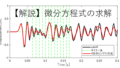
- State variable to be determined: acceleration
Displacements and velocities for all degrees of freedom are obtained, but only the results for the displacement of m10 are presented here.

Figure 2 Acceleration results for m10
In this article, we have briefly explained how to solve the state-space model. The program we used is attached below.
MATLAB code
Executable file
clear all;clc;close all

m_vec=ones(1,10);
k_vec=ones(1,10)*10^5;
[M]=eval_Mmatrix(m_vec); %Mass Matrix
[K]=eval_Kmatrix(k_vec); %Stiffness Matrix
C=K*10^-5;

[V,D]=eig(K,M); %eigenvalue D、eigen vector V
wn=sqrt(diag(D)); %Eig Anguler Freq.
fn=wn/(2*pi); %Eig Freq.


% % Equation of state (continuous time system)
% % dx/dt =Ac x(t) + Bc p(t)
Ac=[zeros(size(M)) eye(size(M))
    -inv(M)*K -inv(M)*C];
Bc=[zeros(size(M))
    -inv(M)];

Cc=[-inv(M)*K -inv(M)*C];

x0 = zeros(size(M,1)*2,1);
x0(1) =1;
t0 = 0;
dt=1/400;
tf = 10;
time=t0:dt:tf;

[T,Y] = ode45(@state_equation, time, x0);
figure
subplot(211)
plot(T,Y(:,10))
xlabel('Time [s]')
ylabel('Displacement [m]')
subplot(212)
y_k=Cc*Y.';
plot(T,y_k(10,:))
xlabel('Time [s]')
ylabel('Acc. [m/s^2]')
functionファイル
function [M]=eval_Mmatrix(m_vec)

M=diag(m_vec);

end
function [K]=eval_Kmatrix(k_vec)

K=zeros(length(k_vec));
for ii1=1:length(k_vec)
    if ii1==1
        K(ii1,ii1)=k_vec(ii1);
    else
        K(ii1-1:ii1,ii1-1:ii1)=K(ii1-1:ii1,ii1-1:ii1)+[1 -1;-1 1]*k_vec(ii1);
    end
end

end
function dx=state_equation(t,x)


m_vec=ones(1,10);
k_vec=ones(1,10)*10^5;
[M]=eval_Mmatrix(m_vec); %Mass Matrix
[K]=eval_Kmatrix(k_vec); %Stiffness Matrix
C=K*10^-5;

% % Equation of state (continuous time system)
% % dx/dt =Ac x(t) + Bc p(t)
Ac=[zeros(size(M)) eye(size(M))
    -inv(M)*K -inv(M)*C];
Bc=[zeros(size(M))
    -inv(M)];

% Cc=[-Sa*inv(M)*K -Sa*inv(M)*C];
% Dc=Sa*inv(M);
p=zeros(size(M,1),1);
% size(p)
% size(Bc)
% size(Bc*p)
%
% size(Ac)
% size(Ac*x)
dx=Ac*x+Bc*p;
end
コメント