
Introduction
I am re-reviewing the bible-like book “Introduction to Modal Analysis,” which every Japanese vibration engineer has read at least once.
I would like to explain what you have learned in the re-review, showing the MATLAB code. This time, I will review from p. 362 of ” Differential Iteration Method” in section 6.3.1. However, the explanation of ” Differential Iteration Method” in “Introduction to Modal Analysis” is very thin and does not include Differential Iteration Method equations, so I will refer to “Modal Analysis and Control of Sound and Vibration” written by Dr. Nagamatsu and others. The chapter I referred to is the commentary by Dr. Yoshimura of Tokyo Metropolitan University. Incidentally, Dr. Yoshimura is a student of Dr. Nagamatsu and is said to be the first person in Japan to conduct research on mode identification (he wrote his doctoral dissertation on mode identification methods).
Differential Iteration Method is the basic idea behind experimental modal analysis and mode identification methods. There are a variety of mode identification methods, but most of them employ the theory of partial iteration method for identification of the distillation number. (Note, however, that mode identification methods are black boxed in experimental modal analysis software, so you will need to ask technical support for the software to answer your questions.)
The following link is a summary to a description of vibration theory in English, if you are interested.

I’ve also developed my own curve fitting software.
If you’re interested, feel free to download it from the link below and give it a try.
👉 Free Download
4.4.1 Differential Iteration Method
In previous articles, you have explained that FRFs and vibration shapes can be expressed as a superposition of modal characteristics (resonant frequencies & vibration modes, etc.). You understand that this concept is modal analysis. And extracting mode characteristics from FRFs is called mode identification.
The mode circle fitting (curve fit) and half width method were applicable only when the adjacent resonance frequencies are far enough apart, as shown in the red frequency band in Figure 1, and the system can be regarded as a one-degree-of-freedom system.
 Figure 1 FRF
On the other hand, the partial iteration method is a mode identification method for multi-degree-of-freedom systems. In other words, this method can extract the mode characteristics of each resonance frequency even if it contains multiple resonance frequencies, such as the 0 to 100 Hz data in Figure 1.
In the previous article, I explained Prony’s method, but Prony’s method was a time-domain (impulse response data) method. The partial iteration method described in this article is a frequency-domain method.
Let us consider the frequency response function between point i and point j. The frequency response function can be expressed as in Equation (4.6).
$$
G_{ij}(ω)=\sum_{r=1}^{n} \left( \frac{ a_r }{ j(ω-s_r)} + \frac{ a^*_r }{ j(ω-s^*_r)} \right) +\frac{Y}{ω^2}+Z \tag{4.6}
$$
ar denotes residu and sr denotes the eigenvalue. the eigenvalue of sr is given by equation (4.2) using the modal damping factor σr and the damped eigenfrequency ωdr.
$$
s_r=-σ_r+jω_{dr} \tag{4.2}
$$
Assuming that the distn ar in Eq. (4.6) is a complex number, it can be decomposed into real and imaginary parts as in Eq. (4.7).
$$
a_r=U_r+jV_r \tag{4.7}
$$
Then equation (4.6) can be rewritten as equation (4.38).
$$
G_{ij}(ω)=\sum_{r=1}^{n} \left( \frac{ U_r+jV_r }{ σ_r + j(ω-ω_{dr})} + \frac{ U_r-jV_r }{ σ_r + j(ω+ω_{dr})} \right) +\frac{Y}{ω^2}+Z \tag{4.38}
$$
Note that Y/ω^2 is a parameter used to correct for frequencies lower than the resonant frequency of symmetry (the resonant frequency of the lowest order for which the mode is being identified), and is called the modulus of mass. On the other hand, Z is the parameter used to correct for frequencies higher than the resonant frequency of symmetry, and is called the modulus stiffness.
Equation (4.38) is divided into real and imaginary parts.
Real Part
$$
G^R_{ij}(ω)=\sum_{r=1}^{n} \left( \frac{ U_r σ_r+jV_r(ω-ω_{dr}) }{ σ_r^2 + (ω-ω_{dr})^2} + \frac{ U_r σ_r-V_r(ω+ω_{dr}) }{ σ_r^2 + (ω+ω_{dr})^2} \right) +\frac{Y}{ω^2}+Z \tag{4.39.1}
$$
Imaginary Part
$$
G^I_{ij}(ω)=\sum_{r=1}^{n} \left( \frac{ -U_r (ω-ω_{dr})+V_rσ_r }{ σ_r^2 + (ω-ω_{dr})^2} – \frac{ U_r (ω+ω_{dr})+V_rσ_r }{ σ_r^2 + (ω+ω_{dr})^2} \right) \tag{4.39.2}
$$
Up to the above, we have been talking about the development of the theoretical equation for the frequency response function.
For convenience, let us express the measured frequency response function E as follows.
(This is to confirm that the frequency response function can be expressed in complex numbers, so it can be divided into real and imaginary numbers.)
$$
E(ω)=E^R(ω)+jE^I(ω)
$$
This is where the idea of the partial iteration method comes in. If the measured frequency response function E can be expressed in terms of the theoretical frequency response function Gij, then the modal characteristics (resonance frequency, modal damping ratio, and frequency fraction) can be obtained, right? Then, the partial iteration method uses the least-squares method to find Ur, Vr, ωdr, and σr of Gij such that the error between E and Gij is minimized.
In other words, the evaluation function λ (sum of squares of errors) becomes equation (4.40.0).
$$
λ=\sum_{ω=ω_{start}}^{ω_{end}} \left( (E^R(ω)-G^R_{ij}(ω))^2 + (E^I(ω)-G^I_{ij}(ω))^2 \right) \tag{4.40.0}
$$
However, equation (4.40.0) does not work. This is because the response at resonant frequencies can be hundreds to thousands of times larger than the response at non-resonant frequencies. This means that the evaluation function λ in Eq. (4.40.0) should just identify Ur, Vr, ωdr, and σr such that only the values at the resonant frequency match. This is not good enough. Generally, we would like to identify frequency response functions that also match the actual measurement in frequency bands other than the resonant frequency.
Therefore, we introduce a weight function W(ω) to the evaluation function λ, as in Eq. (4.40).
$$
λ=\sum_{ω=ω_{start}}^{ω_{end}} \left( (E^R(ω)-G^R_{ij}(ω))^2 + (E^I(ω)-G^I_{ij}(ω))^2 \right)W(ω) \tag{4.40}
$$
From here on, the notation is changed as follows to represent it in matrix form.
$$
E=\left(
\begin{array}{c}
E^R(ω_{start}) \\
\vdots \\
E^R(ω_{end}) \\
E^I(ω_{start}) \\
\vdots \\
E^I(ω_{end})
\end{array}
\right) ,
G=\left(
\begin{array}{c}
G^R_{ij}(ω_{start}) \\
\vdots \\
G^R_{ij}(ω_{end}) \\
G^I_{ij}(ω_{start}) \\
\vdots \\
G^I_{ij}(ω_{end})
\end{array}
\right) ,
W=\begin{pmatrix}
W(ω_{start}) & & & & & \\
& \ddots & & \Huge{0} & & \\
& & W(ω_{end}) & & & \\
& \Huge{0} & & W(ω_{start}) & & \\
& & & & \ddots & \\
& & & & & W(ω_{end})
\end{pmatrix} \tag{4.41}
$$
Using the weight function matrix in equation (4.41), the evaluation function λ is replaced as in equation (4.42).
$$
λ=[\bf{E-G}]^t \bf{W} [\bf{E-G}] \tag{4.42}
$$
Now, we can define the evaluation function λ. Again, the evaluation function λ is the error between the measured and theoretical values. So, we can find Ur, Vr, ωdr, and σr such that the evaluation function λ is minimized. To find Ur, Vr, ωdr, and σr such that the evaluation function λ is minimized, it is sufficient to find parameters such that the partial derivative of λ is zero for each parameter.
For now, let us assume that Ur, Vr, ωdr, and σr are design variables a and obtain the following.
$$
\frac{\partial λ}{\partial \bf{a}} = -2 [ \frac{\partial \bf{G}}{\partial \bf{a}} ]^t \bf{W} [\bf{E-G}] = \bf{0} \tag{4.44}
$$
Since we just summarized the design variables as a, you may be asking, “What exactly is ∂G/∂a?” You may be wondering, “What is ∂G/∂a? For example, by replacing a with Ur and then performing partial differentiation, we can obtain the partial derivative of each parameter. (The equation gets a little complicated, so I will paste it in an image.)

Let ao be the initial value design variable, and Taylor expansion of Equation (4.44) at ao, omitting terms after the second order, yields Equation (4.47).
$$
\bf{G(a)}=\bf{G(a_0)}+[\frac{\partial \bf{G}}{\partial \bf{a}}]\bf{δa} \tag{4.47}
$$
Substituting equation (4.47) into equation (4.44) yields equation (4.49).
$$
[ \frac{\partial \bf{G}}{\partial \bf{a}} ]^t \bf{W} [\bf{E-G(a_0)}] = [\frac{\partial \bf{G}}{\partial \bf{a}}]^t \bf{W} [\frac{\partial \bf{G}}{\partial \bf{a}}]\bf{δa} \tag{4.49}
$$
式(4.49)および式(4.47)は初期値aoでテイラー展開で線形近似して求めたので、初期値を設定する必要があります。またテイラー展開は初期値近傍において線形性が保たれるので、初期値aoから微小にa=ao+δaとして更新していくことになります。
Equations (4.49) and (4.47) were obtained by linear approximation using Taylor expansion with an initial value of ao, so it is necessary to set an initial value. In addition, since the Taylor expansion maintains linearity in the vicinity of the initial value, a = ao + δa is updated from the initial value of ao in minute increments.
Now, please review the flowchart that shows the equations up to this point and the method for identifying the mode parameters (Ur, Vr, ωdr, and σr). The linear and nonlinear terms in the figure correspond to the numerator (linear term) and denominator (nonlinear term) of equation (4.6).

Figure (Sorry I have no time to translate….)
With the theory explained here, we will continue the explanation through examples.
Example
Consider the following frequency response function for a 4-DOF spring-mass system with a modal damping ratio of 4%.

Let the above be the measured frequency response function E. By the way, the true resonance frequency ωdr and the modal damping ratio ζ are in the table below.
| 1st | 2nd | 3rd | 4th | |
| ωdr | 34.73 | 100.00 | 153.21 | 187.94 |
| ζ | 4.00% | 4.00% | 4.00% | 4.00% |
When using the partial iteration method for identification, initial values must be set. The initial values of ωdr are roughly 30 Hz, 95 Hz, 155 Hz, and 190 Hz from the graph. Since the modal damping cannot be read from the graph, it is assumed to be 10% for the time being.
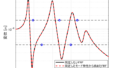
The following is the result of identifying the mode characteristics and recalculating the frequency response function according to the flowchart in the figure.

I see that the recalculated frequency response function is consistent with the FRF we want to identify (the measured FRF).
The identified modal parameters are shown in the table below.
| 1st | 2nd | 3rd | 4th | |
| ωdr | 34.70 | 99.91 | 153.03 | 187.77 |
| σr | 1.39 | 4.02 | 6.19 | 7.31 |
| ζ | 4.01% | 4.03% | 4.04% | 3.89% |
| Ur | 1.29E-07 | 3.03E-07 | 7.88E-06 | 8.28E-07 |
| Vr | -7.49E-04 | -1.67E-03 | -1.41E-03 | -4.79E-04 |
I see that the modal damping ratio ζ is almost 4% and the resonance frequency ωdr can be estimated with little error. With this program, you will be able to perform mode identification without expensive vibration measurement software.
MATLAB code
Executable program
clear all;clc;close all

freq=0.1:0.1:40; %Definition of calculation frequency
df=freq(2) - freq(1);
w=2*pi*freq; %Angular frequency
m_vec=ones(1,4);
k_vec=ones(1,4)*10^4;
[M]=eval_Mmatrix(m_vec); %mass matrix
[K]=eval_Kmatrix(k_vec); %stiffness matrix

[V,D]=eig(K,M); % eigenvalue D, eigenvector V
for ii1=1:length(m_vec)
    V(:,ii1)=V(:,ii1)/V(1,ii1); % normalize so that the component of mode vector at excitation point m1 is 1
end
wn=sqrt(diag(D)); % natural angular frequency
fn=wn/(2*pi); % natural frequency

mr=diag(V.'*M*V); %mode mass matrix
kr=diag(V.'*K*V); %mode stiffness matrix
c_cr=2*sqrt(mr.*kr);
modal_dampimg=1*0.04; % modal damping ratio (set to 4% for now)
cr=c_cr*modal_dampimg; %mode damping factor

F=zeros(length(m_vec),1); F(1)=1; %external force vector (all frequency bands are vibrated by 1)
Xj=zeros(length(m_vec),length(freq)); %displacement vector (define vector and allocate memory before calculation)

% % % mode method
ii=1; %excitation points (if there are multiple excitation points, just add a loop for ii=1:kength(F))
for ii1=1:length(m_vec) %response point
    for ii2=1:length(wn)
        Xj(ii1,:)=Xj(ii1,:)+V(ii1,ii2)*V(ii,ii2)./( -mr(ii2).*w.^2 + 1i*cr(ii2)*w +kr(ii2) )*F(ii);
    end
end

FRF_E=Xj(1,:);


figure
semilogy(w,abs(FRF_E),'k-','linewidth',2)
hold on
xlabel('Angular frequency Hz')
label('Displacement [m]')
xlim([w(1) w(end)])
grid on


%%%%%%%%%%%%%%%%%%%%%%%%%%%%%%%%%%%%%%%%%%%%%%%%%%%%%%%%%%%%%%%%%%%%%%%%%%%%%%%%%%
%%%%%%%%%%%%%%%%%%%%%%%%%%%%%%%%%%%%%%%%%Differential Iteration Method
%%%%%%%%%%%%%%%%%%%%%%%%%%%%%%%%%%%%%%%%%%%%%%%%%%%%%%%%%%%%%%%%%%%%%%%%%%%%%%%%%%
N=100; %Number of iterations
wdr=[30 95 155 190]; %initial value wdr
sigma_r=wdr*0.1; %initial value of σr, σr=angular resonance frequency x mode damping ratio

[Ur,Vr,Y,Z,wdr,sigma_r,modal_damp,G]=Differential_Iteration_Method(N,FRF_E,w,wdr,sigma_r);


semilogy(w,abs(G(1:length(w))+j*G(length(w)+1:end)),'r--','linewidth',2)
legend('FRF to be identified (FRF of actual measurement)','FRF after 100 searches')
functionファイル
function [Ur,Vr,Y,Z,wdr,sigma_r,modal_damp,G]=Differential_Iteration_Method(N,FRF_E,w,wdr,sigma_r)

if N==1
    N=2;
end

lambda=zeros(1,N);
E=[real(FRF_E),imag(FRF_E)].'; % Measured FRF matrix E
W=diag(1./[abs(FRF_E) abs(FRF_E)]).^2; %The weight function matrix W
Nmode=length(wdr);

%%%%%%%%%%%%%%%%%%%%%%%%%%%%%%%%%%%%%%%%% Calculation of linear terms
[dGdaLiner]=dGdaLiner_Matrix(wdr,sigma_r,w,Nmode); eq式(4.45)
aLiner=inv(dGdaLiner.'*W*dGdaLiner)*dGdaLiner.'*W*E;%eq(4.44)  & G=dGdaLiner*aLiner
G=dGdaLiner*aLiner; %Recalculation of frequency response function
lambda(1,1)=(E-G).'*W*(E-G);

for ii1=2:N
% %%%%%%%%%%%%%%%%%%%%%%%%%%%%%%%%%%%%%%%%% Update nonlinear terms
    Ur=aLiner(1:Nmode); Vr=aLiner(Nmode+1:Nmode*2);
    [dGdaNONLiner]=dGdaNONLiner_Matrix(Ur,Vr,wdr,sigma_r,w,Nmode); %eq(4.45)
    aNONLiner=[sigma_r wdr].';
    da=inv(dGdaNONLiner.'*W*dGdaNONLiner)*dGdaNONLiner.'*W*(E-G); %eq(4.49)
    aNONLiner = aNONLiner + da; %eq(4.46)
    modal_damp=aNONLiner(1:Nmode)./aNONLiner(Nmode+1:Nmode*2);
%%%%%%%%%%%%%%%%%%%%%%%%%%%%%%%%%%%%%%%%% Calculation of linear terms
sigma_r=aNONLiner(1:Nmode).';  wdr=aNONLiner(Nmode+1:Nmode*2).';
[dGdaLiner]=dGdaLiner_Matrix(wdr,sigma_r,w,Nmode); %eq(4.45)
aLiner=inv(dGdaLiner.'*W*dGdaLiner)*dGdaLiner.'*W*E; %eq(4.44)  & G=dGdaLiner*aLiner
G=dGdaLiner*aLiner; %Recalculation of frequency response function
lambda(1,ii1)=(E-G).'*W*(E-G);
end

G=dGdaLiner*aLiner;

% % % Final Results
Ur=aLiner(1:Nmode);
Vr=aLiner(Nmode+1:Nmode*2);
Y=aLiner(Nmode*2+1);
Z=aLiner(Nmode*2+2);
sigma_r=aNONLiner(1:Nmode).';
wdr=aNONLiner(Nmode+1:Nmode*2).';
modal_damp=sigma_r./wdr;

end
function [M]=eval_Mmatrix(m_vec)

M=diag(m_vec);

end
function [K]=eval_Kmatrix(k_vec)

K=zeros(length(k_vec));
for ii1=1:length(k_vec)
    if ii1==1
        K(ii1,ii1)=k_vec(ii1);
    else
        K(ii1-1:ii1,ii1-1:ii1)=K(ii1-1:ii1,ii1-1:ii1)+[1 -1;-1 1]*k_vec(ii1);
    end
end

end
function [dGdaLiner]=dGdaLiner_Matrix(wdr,sigma_r,w,Nmode)

% w=2*pi*freq;
Re_T=zeros(length(w),2*Nmode);
Im_T=zeros(length(w),2*Nmode);

for ii1=1:length(w)
    for ii2=1:Nmode
        Ar=sigma_r(ii2)^2+(w(ii1)-wdr(ii2))^2;
        Br=sigma_r(ii2)^2+(w(ii1)+wdr(ii2))^2;
        Cr=-sigma_r(ii2)^2+(w(ii1)-wdr(ii2))^2;
        Dr=-sigma_r(ii2)^2+(w(ii1)+wdr(ii2))^2;
        % σr
        Re_T(ii1,ii2)= ( Ur(ii2)*Cr-2*Vr(ii2)*(w(ii1)-wdr(ii2)) )*sigma_r(ii2)/Ar^2 +......
                       ( Ur(ii2)*Dr+2*Vr(ii2)*(w(ii1)+wdr(ii2)) )*sigma_r(ii2)/Br^2;
        % ωdr
        Re_T(ii1,ii2+Nmode)= ( Vr(ii2)*Cr+2*Ur(ii2)*(w(ii1)-wdr(ii2)) )*sigma_r(ii2)/Ar^2 +......
                             ( Vr(ii2)*Dr-2*Ur(ii2)*(w(ii1)+wdr(ii2)) )*sigma_r(ii2)/Br^2;
        % σr
        Im_T(ii1,ii2)= ( Vr(ii2)*Cr+2*Ur(ii2)*(w(ii1)-wdr(ii2)) )*sigma_r(ii2)/Ar^2 +......
                       ( -Vr(ii2)*Dr+2*Ur(ii2)*(w(ii1)+wdr(ii2)) )*sigma_r(ii2)/Br^2;
        % ωdr
        Im_T(ii1,ii2+Nmode)= ( -Ur(ii2)*Cr+2*Vr(ii2)*(w(ii1)-wdr(ii2)) )*sigma_r(ii2)/Ar^2 +......
                             ( Ur(ii2)*Dr+2*Vr(ii2)*(w(ii1)+wdr(ii2)) )*sigma_r(ii2)/Br^2;
    end
end
dGdaNONLiner=[Re_T
    Im_T];
end
コメント