Introduction
We often hear that “averaging can reduce the effect of noise.”
However, people who do not handle actual measurement data (people who do not conduct experiments) do not really understand this. The reason is that there is no error in the data we are dealing with in the first place.
In this article, I would like to explain noise reduction (error reduction) by averaging. This is the first article on “averaging,” so it is intended to give those who are studying averaging for the first time an idea of what it is all about. In the next and subsequent articles, I will introduce more technical details.
If you want to see all my lessons in English, please see below.

Type of Noise
Broadly speaking, there are two types of noise that we deal with in the vibration and noise field.
The first is uncorrelated noise. Uncorrelated noise is noise that has no correlation with the signal to be measured.
The second is periodic noise. Power supply noise and fan noise are examples of periodic noise.
Uncorrelated noise (random noise)
To explain it super simply, a signal using the rand function in MATLAB is “uncorrelated noise”.
・MATLAB code
clc;clear all;close all
fs=1024;
t=linspace(0,1,fs+1);
rand_sig=2*(rand(1,fs+1)-0.5);

figure
plot(t,rand_sig)
xlabel('時間 [s]')
ylabel('音圧 [Pa]')
Periodic noise
Periodic noise refers to power supply noise and fan noise.
It is difficult for those who have never experimented to understand, but most machines are equipped with electronics. This electronics runs on electricity and must be connected to a power source (outlet). When measuring vibration or noise, noise of 50 Hz or 60 Hz, the frequency of the power supply, may be added to the measurement signal.
This noise is called power supply noise. Power supply noise can be reduced by grounding electronic equipment or measuring instruments.
(However, it is quite difficult to reduce power supply noise, and it can take up to a day to do so.)
Fan noise is generated at a frequency of (number of fan blades) x (rotational frequency). This is called fan noise or fan noise.
This is not explained here, but when handling motors, noise called electromagnetic noise may be generated.
Noise reduction by averaging
To conclude first, uncorrelated noise can be reduced by averaging, but periodic noise cannot be reduced by averaging.
Uncorrelated noise (random noise)
Now, I would like to explain with the help of an example.
〇Example
Suppose that the signal to be observed is buried in “uncorrelated noise. The signal to be measured is uncorrelated noise with the signal to be observed. Extract the signal to be observed from the signal to be measured by averaging. Each signal is assumed to be as follows
Signal to be observed: sin wave of amplitude 0.1 and frequency 10 Hz
Uncorrelated noise: white noise (random noise) of amplitude 1
Now, what do we do?
(As the title says “noise reduction by averaging,” all we have to do is to average the noise. …..)
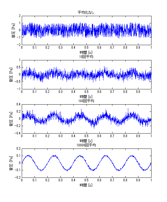
First, let’s check the results without averaging. The figure below shows the result without averaging.
Now, let’s do an average of 10 times. By the way, the code is as follows
・Code
clc;clear all;close all

fs=1024;
t=linspace(0,1,fs+1);

% % % 観測したい信号
sig=0.1*sin(10*pi*t);
% % % 無相関のノイズ1
rand_sig=2*(rand(1,fs+1)-0.5);
% % % 測定信号
measurement_sig1=sig+rand_sig;

% % % 10回平均
measurement_sig2=zeros(10,fs+1);
for ii1=1:10
    rand_sig=2*(rand(1,fs+1)-0.5);
    measurement_sig2(ii1,:)=sig+rand_sig;
end

figure
% subplot(411)
plot(t,measurement_sig1)
xlabel('時間 [s]')
ylabel('音圧 [Pa]')
title('平均化なし')
ylim([-1.2 1.2])

figure
% subplot(412)
plot(t,mean(measurement_sig2))
xlabel('時間 [s]')
ylabel('音圧 [Pa]')
title('10回平均')
ylim([-1.2 1.2])
The result is shown in the figure below.
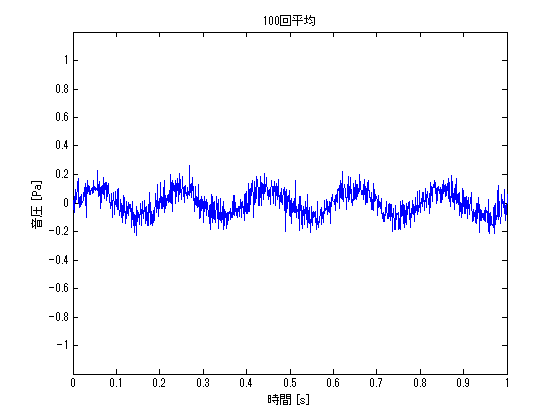
The effect of noise has been reduced, and the characteristics of the sin wave have become a little more apparent. The same procedure is used to check the results of 100 and 10,000 averages.
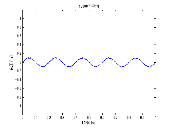
Averaging 10000 times, we can extract a very beautiful sin wave. If the number of averaging times is further increased, a cleaner sin wave can be extracted.
In practical use, the number of averaging times cannot be increased infinitely, so averaging should be done as many times as possible to ensure a sufficient signal-to-noise ratio (signal to noise ratio). (It may be decided at random.)
Periodic noise
Verify the following as in the previous example.
・位相に相関性がある場合
○Example
Signal to be observed: sin wave of amplitude 1 and frequency 10Hz
Periodic noise: sin wave of amplitude 1 and frequency 60Hz
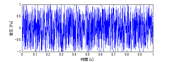
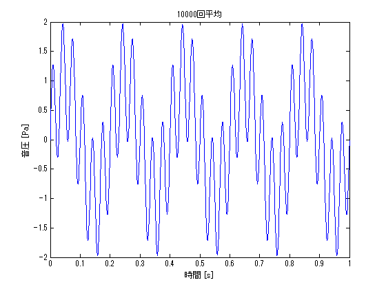
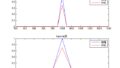
Now, let’s look at the result of averaging over 1000 times. I believe we have confirmed that averaging does not reduce the effect of periodic noise. Averaging has no effect on periodic noise because it uses the fact that uncorrelated values converge to the mean or median value.
・Code
clc;clear all;close all

fs=1024;
t=linspace(0,1,fs+1);

% % % 観測したい信号
sig=1*sin(10*pi*t);

% % % 10000回平均
measurement_sig=zeros(10000,fs+1);
for ii1=1:10000
    % % % 周期性のノイズ
    sig_noise=1*sin(60*pi*t);
    % % % 測定信号
    measurement_sig(ii1,:)=sig+sig_noise;
end

figure
plot(t,mean(measurement_sig))
xlabel('時間 [s]')
ylabel('音圧 [Pa]')
title('10000回平均')
% ylim([-1.2 1.2])
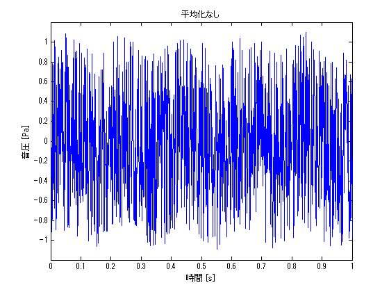
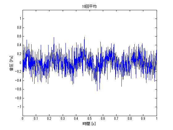
・When phase is uncorrelated
The same example problem as before shows the effect of averaging when the phases are uncorrelated.
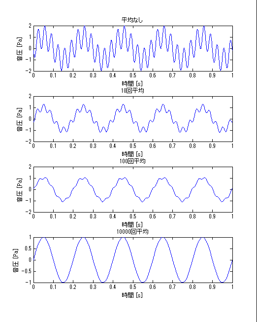
Some of you may be thinking, “Even with periodic noise, the averaging process can reduce the effect of the noise!” I guess some of you are thinking, “Even with periodic noise, the averaging process can reduce the effect of noise! However, this is a very special condition.
Phase uncorrelated” means that the ratio of the phase angle between the “signal to be observed” and the “periodic noise” is different for each averaging frequency. Depending on the test conditions, it is possible to create a state of “phase uncorrelatedness,” but it is not realistic because it is quite time-consuming.
For example, suppose that the sound is emitted from a speaker in a space with noisy fan noise (periodic noise) and measured at the evaluation point. You want to reduce the influence of this fan noise, so you want to make the phase uncorrelated with the speaker.
Under this test condition, we can reduce the fan noise by randomly changing the timing of sound emission from the speaker for each measurement and averaging the measurement results.
We would repeat On-Off of the sound source playback for each measurement so that it is uncorrelated, and make dozens to hundreds of measurements. It is quite a hard task, isn’t it?
・Code
clc;clear all;close all

fs=1024;
t=linspace(0,1,fs+1);

% % % 観測したい信号
sig=1*sin(10*pi*t);
phy=rand(1)*2*pi;
% % % 周期性のノイズ
sig_noise=1*sin(60*pi*t+phy);
% % % 測定信号
measurement_sig1=sig+sig_noise;


% % % 10回平均
measurement_sig2=zeros(10,fs+1);
for ii1=1:10
    % % % 位相
    phy=rand(1)*2*pi;
    % % % 周期性のノイズ
    sig_noise=1*sin(60*pi*t+phy);
    % % % 測定信号
    measurement_sig2(ii1,:)=sig+sig_noise;
end

% % % 100回平均
measurement_sig3=zeros(100,fs+1);
for ii1=1:100
    % % % 位相
    phy=rand(1)*2*pi;
    % % % 周期性のノイズ
    sig_noise=1*sin(60*pi*t+phy);
    % % % 測定信号
    measurement_sig3(ii1,:)=sig+sig_noise;
end

% % % 10000回平均
measurement_sig4=zeros(10000,fs+1);
for ii1=1:10000
    % % % 位相
    phy=rand(1)*2*pi;
    % % % 周期性のノイズ
    sig_noise=1*sin(60*pi*t+phy);
    % % % 測定信号
    measurement_sig4(ii1,:)=sig+sig_noise;
end


figure
subplot(411)
plot(t,measurement_sig1)
xlabel('時間 [s]')
ylabel('音圧 [Pa]')
title('平均なし')
% ylim([-1.2 1.2])

subplot(412)
plot(t,mean(measurement_sig2))
xlabel('時間 [s]')
ylabel('音圧 [Pa]')
title('10回平均')
% ylim([-1.2 1.2])

subplot(413)
plot(t,mean(measurement_sig3))
xlabel('時間 [s]')
ylabel('音圧 [Pa]')
title('100回平均')
% ylim([-1.2 1.2])

subplot(414)
plot(t,mean(measurement_sig4))
xlabel('時間 [s]')
ylabel('音圧 [Pa]')
title('10000回平均')
% ylim([-1.2 1.2])
コメント