Introduction
There are several types of transfer functions (Frequency Response Function (FRF)): H1 estimation, H2 estimation, H3 estimation, and Hv estimation.
So far, we have introduced H1 and H2 estimation. This article describes H3 and Hv estimation.
If you want to see all my lessons in English, please see below.

Some of you may be wondering, “Is there more than one type of FRF(= response/input)?”
Those who have this question do not understand the concept of noise reduction by averaging process; the name of the estimation changes depending on how the averaging process is used when FRF is calculated. Also, there is something else to consider besides the effect of noise.
In the actual measurement, there is a difference between the first (response)/(input) and the second (response)/(input).
(In analysis, the first and second are the same.)
It is difficult to say why the difference occurs in the actual measurement, since there are various causes, but the following are typical examples.
FRF is measured by hammering test → Varying excitation force → Effect of excitation force dependence becomes apparent.
FRF is measured in a hammering test → FRF becomes more stable with time (influence of screw fixation, etc.) → Frequency response changes.
There are many causes, but since FRF varies from one measurement to another, there is an evaluation index that indicates how reliable it is, which is called the coherence function.
Today we will discuss H1 estimation.
Next time, I will discuss H2 estimation, then H3 estimation, Hv estimation, and the coherence function in turn.
H1 estimation of FRF
As mentioned earlier, there are several types of FRFs: H1 estimation, H2 estimation, and Hv estimation. Of these, H1 estimation is the most common method of estimating the transfer function.
First, let us consider the ideal FRF. The ideal FRF G(ω) is as follows

(入力=input、応答=response)
However, as a practical matter, such ideal measurement is not possible. This is because of the influence of noise.
For example, in an acoustic measurement using a speaker, the input signal is the voltage of the speaker and the response is the sound measured by the microphone. But the sound will contain background noise (noise), right?
As in this example, it is often the case that the input signal has a small effect of noise, but the response signal has an effect of noise. (Or the effect of noise on the response signal is unknown)
The above example is represented as a block diagram in the figure below.

(入力=input、応答=response、ノイズ=noise)
The H1 estimation is a method to estimate FRF = (response V)/(input F) in a situation where the response signal contains noise components, as shown in the figure above.
Theory of H1 Estimation
The formula for H1 estimation in the textbook itself is very simple. The theoretical formula is based on the following.
$$
H1(ω)= \frac{W_{fx}(ω)}{W_{ff}(ω)}
$$
where Wfx is the Cross Spectral Density Function of F and X, and Wff is the Power Spectral Density Function or Auto Spectral Density Function.
However, the formula for Hz estimation in the textbook is a bit wrong. It is actually the following, where N is the number of times of averaging.
$$
H1(ω)= \frac{\sum_{n=1}^{N} W_{fx}(ω)}{\sum_{n=1}^{N} W_{ff}(ω)}
$$
Or (what I mean below is that it can be obtained from the average of the cross spectral density function and the average of the power spectral density function)
$$
H1(ω)= \frac{\sum_{n=1}^{N} W_{fx}(ω)/N}{\sum_{n=1}^{N} W_{ff}(ω)/N}
$$
Now we will explain why the above equation can reduce noise in the response.
Note that * refers to conjugation.
$$
H1(ω)= \frac{\sum_{n=1}^{N} F(ω)^*X(ω)}{\sum_{n=1}^{N} F(ω)^*F(ω)}
$$
$$
H1(ω)= \frac{\sum_{n=1}^{N} F(ω)^*(V(ω)+N(ω))}{\sum_{n=1}^{N} F(ω)^*F(ω)}
$$
$$
H1(ω)= \frac{\sum_{n=1}^{N} (F(ω)^*V(ω)+F(ω)^*N(ω))}{\sum_{n=1}^{N} F(ω)^*F(ω)}
$$
Since the noise component N is assumed to be uncorrelated noise, the averaging process brings it close to 0.
Therefore, when N is increased and averaged, the uncorrelated noise N converges to 0, resulting in the formula below.
$$
H1(ω)= \frac{\sum_{n=1}^{N} F(ω)^*V(ω)}{\sum_{n=1}^{N} F(ω)^*F(ω)}
$$
Noise can be reduced by the above.
Validation in MATLAB
Result
The results of the analysis are shown first. (100 times average)
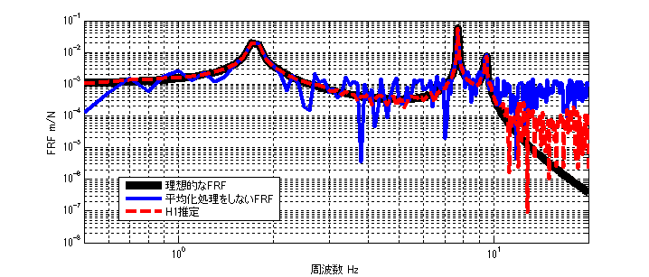
The ideal FRF with no noise component is shown by the black line.
The FRF with noise components and without averaging is represented by the blue line, and
(The H1 estimation result (with averaging) is shown by the red dotted line.
As can be seen from the figure, the error between the ideal FRF and the H1 estimation result is smaller than that of the FRF without averaging.
Incidentally, since the noise component is given at 5% of the maximum amplitude of response X, it can be seen that at frequencies where response X was originally small (e.g., above 10 Hz), the noise component is relatively large, so it is difficult to reduce the noise even after averaging.
MATLAB code
Executable file
clear all
close all
% % % % 初期設定
freq=0.5:0.1:20;
m_vec=[1 1 1 1];
[M]=eval_Mmatrix(m_vec);
k_vec=[1 1 1 1]*10^3;
[K]=eval_Kmatrix(k_vec);
C=zeros(length(k_vec));
F=zeros(length(m_vec),length(freq));
F(1,:)=ones(1,length(freq));

% % % % 変位X(ノイズなし)
X=eval_direct_x_2ndedition(M,K,C,F,freq);
% % % % 理想的なFRF
FRF_ideal_x3_f1=X(3,:)./F(1,:);

N=100; %平均化回数 100回
res=zeros(N,length(freq));
ref=zeros(N,length(freq));
for ii1=1:N
    res(ii1,:)=X(3,:)+( rand(1,length(freq)) - 0.5 )*max(abs(X(3,:)))*0.05; % 最大変位Xを基準として5%のノイズを加える
    ref(ii1,:)=F(1,:);
end

[h1] = H1(ref,res,freq);

figure(1)
loglog(freq,abs(FRF_ideal_x3_f1),'k','linewidth',7)
hold on
loglog(freq,abs(res(1,:)./ref(1,:)),'b','linewidth',3)
loglog(freq,abs(h1),'r--','linewidth',3)
hold off
grid on
legend('理想的なFRF','平均化処理をしないFRF','H1推定')
xlim([freq(1) freq(end)])
xlabel('周波数 Hz');ylabel('FRF m/N');
function file
function [K]=eval_Kmatrix(k_vec)
K=zeros(length(k_vec));
for ii1=1:length(k_vec)
    if ii1==1 K(ii1,ii1)=k_vec(ii1);
    else
        K(ii1-1:ii1,ii1-1:ii1)=K(ii1-1:ii1,ii1-1:ii1)+[1 -1;-1 1]*k_vec(ii1);
    end
end

end
function [M]=eval_Mmatrix(m_vec)
M=diag(m_vec);
end
function x=eval_direct_x_2ndedition(M,K,C,F,freq)
% % 2021.05.28 Fを修正
x=zeros(size(F,1),length(freq));
j=sqrt(-1);
for ii1=1:1:length(freq)
    w=2*pi*freq(ii1);
    x(:,ii1)=inv(K+j*w*C-w^2*M)*F(:,ii1);
end

end
function [Wff]=PowerSpectralDensity(F,freq)

if size(F,1)==length(freq)
    F=F.';
end

Wff=conj(F).*F;


end
function [Wfx]=CrossSpectralDensity(F,X,freq)

if size(F,1)==length(freq)
    F=F.';
end
if size(X,1)==length(freq)
    X=X.';
end


Wfx=conj(F).*X;


end
function [h1] = H1(ref,res,freq)

% h1=zeros(1,freq);

[Wfx]=CrossSpectralDensity(ref,res,freq);
[Wff]=PowerSpectralDensity(ref,freq);

h1=mean(Wfx,1)./mean(Wff,1);

end
コメント