
Introduction
We have previously described mode circle fitting, the Prony method (polyreference method), and the partial fraction iteration method. In this article, I will explain the mode identification method called the Rational Fraction Polynomial Method.
My favorite book on vibration engineering, “Introduction to Modal Analysis,” does not cover the mode identification method sufficiently. Therefore, I will introduce some Japanese and foreign books in which the RFP method is introduced.
The RFP method is described in “Method II: Rational Fraction Polynomial Method (RFP)” in section 4.4.3 of the book “Modal Tesiting” by Ewin.
If you want to see all my lessons in English, please see below.

I’ve also developed my own curve fitting software.
If you’re interested, feel free to download it from the link below and give it a try.
👉 Free Download
4.4.3 RFP Method
※This article corresponds to the formulas in “Modal Tesiting”and “Modal Analysis and Control of Sound and Vibration(「音・振動のモード解析と制御」)”.
Mathematical formulas cited from “Modal Testing” are marked with MT at the end, and those from “Modal Analysis and Control of Sound and Vibration” are marked with OT. Please note that the formulas are cited across references, so there may be inconsistencies in symbols in some places.
The characteristics of RFP express the transfer function H as in the IIR filter as in the equation below.
$$
H(ω)= \frac{ b_0 + b_1(iω) + b_2(iω)^2 + \cdots + b_{2N-1}(iω)^{2N-1} }{ a_0 + a_1(iω) + a_2(iω)^2 + \cdots + a_{2N}(iω)^{2N} } \tag{4.38MT}
$$
It is good that the transfer function H can be expressed as in equation (4.38MT), but how to obtain the coefficients of an and bn from the actual measured transfer function?
This is where the mode identification method becomes difficult.
Suppose we first tentatively determine the coefficients an and bn in equation (4.38). Then, if the value of the transfer function for the actual measurement of angular frequency ωk is Hk, the error ek is as in equation (4.39aMT).
$$
ek= \frac{ b_0 + b_1(iω_k) + b_2(iω_k)^2 + \cdots + b_{2N-1}(iω_k)^{2N-1} }{ a_0 + a_1(iω_k) + a_2(iω_k)^2 + \cdots + a_{2N}(iω_k)^{2N} }-H_k \tag{4.39aMT}
$$
For convenience in future calculations, we transform Equation (4.39aMT) into Equation (4.39bMT).
$$
ek’= (b_0 + b_1(iω_k) + b_2(iω_k)^2 + \cdots + b_{2N-1}(iω_k)^{2N-1}) – H_k ( a_0 + a_1(iω_k) + a_2(iω_k)^2 + \cdots + a_{2N}(iω_k)^{2N} ) \tag{4.39bMT}
$$
Equation (4.39bMT) is expressed in matrix form as Equation (4.41aMT).
$$
ek’=\left( \begin{array}{ccccc}
1 & (iω_k) & (iω_k)^2 & \cdots & (iω_k)^{2N-1}
\end{array} \right)
\left( \begin{array}{c}
b_0 \\
\vdots \\
b_{2N-1}
\end{array} \right) -H_k
\left( \begin{array}{ccccc}
1 & (iω_k) & (iω_k)^2 & \cdots & (iω_k)^{2N-1}
\end{array} \right)
\left( \begin{array}{c}
a_0 \\
\vdots \\
a_{2N-1}
\end{array} \right)-Hk(iω_k)^{2N} a_{2m} \tag{4.41aMT}
$$
Since this is the error ek at ωk, the following equation is given in matrix notation so that it can be applied in the frequency band. Note that from this point forward, the equation is taken from the 1982 IMAC paper.
$$
e=\left( \begin{array}{ccccc}
1 & (iω_1) & (iω_1)^2 & \cdots & (iω_1)^{2N-1} \\
\vdots & \vdots & \vdots & \vdots & \vdots \\
1 & (iω_L) & (iω_L)^2 & \cdots & (iω_L)^{2N-1}
\end{array} \right)
\left( \begin{array}{c}
b_0 \\
\vdots \\
b_{2N-1}
\end{array} \right) –
\left( \begin{array}{ccccc}
H_1 & H_1(iω_k) & H_1(iω_k)^2 & \cdots & H_1(iω_k)^{2N-1} \\
\vdots & \vdots & \vdots & \vdots & \vdots \\
H_L & H_L(iω_k) & H_L(iω_k)^2 & \cdots & H_L(iω_k)^{2N-1}
\end{array} \right)
\left( \begin{array}{c}
a_0 \\
\vdots \\
a_{2N-1}
\end{array} \right)-
\left( \begin{array}{c}
H_1(iω_k)^{2N} \\
\vdots \\
H_L(iω_k)^{2N}
\end{array} \right)
\tag {4.1000}
$$
The matrix notation of equation (4.1000) becomes equation (4.1001).
$$
[ε]=[P][B] -[T][A] – [W] \tag{4.1001}
$$
Since the parameters are to be identified so as to minimize this error vector ε, the following evaluation function λ is to be minimized. (εk is a vector notation of ε.)
$$
λ=[ε]^H [ε] \tag{4.1002}
$$
Since we want to find [A] and [B] such that the evaluation function λ is minimized, the following evaluation function λ is to be differentiated by [A] and [B].
$$
\frac{\partial λ}{\partial [A]}=0 , \frac{\partial λ}{\partial [B]}=0
$$
Solving the above equation yields equation (4.1003).
$$
\left( \begin{array}{cc}
Re([P]^H [P]) & Re([P]^H [T]) \\
Re([P]^H [T])^t & Re([T]^H [T])
\end{array} \right)
\left( \begin{array}{c}
[B] \\
[A]
\end{array} \right) =
\left( \begin{array}{c}
Re([P]^H [W]) \\
-Re([T]^H [W])
\end{array} \right) \tag{4.40MT}
$$
Equation (4.40MT) becomes unsolvable due to the bad condition of the matrix. Therefore, equation (4.40MT) must be rewritten.
$$
H(ω_i)=\frac{\sum_{k=0}^{m} c_k φ_{i.k} } {\sum_{k=0}^{n} d_k θ_{i.k} } \tag{4.60OT}
$$
It is important to start here.
Suppose that φkr and θkr in equation (4.60OT) are r-th order orthogonal polynomials and have characteristics like the orthogonality of the modes as shown in equations (4.61OT) and (4.62OT).
\[
\sum_{k=1}^{m} φ_{i.k}^* φ_{i.j}=
\left\{
\begin{array}{l}
0 & (k≠j)\\
0.5 & (k=j)
\end{array}
\right. \tag{4.61OT}
\]
\[
\sum_{k=1}^{m} θ_{i.k}^* |E(ω_i)|^2 θ_{i.j}=
\left\{
\begin{array}{l}
0 & (k≠j)\\
0.5 & (k=j)
\end{array}
\right. \tag{4.62OT}
\]
The error vector is shown in the same way as in equation (1000).
$$
ε=
\left( \begin{array}{ccc}
φ_{ 1,0 } & \ldots & φ_{ 1,m } \\
\vdots & \ddots & \vdots \\
φ_{ L,0 } & \ldots & φ_{ L,m }
\end{array} \right)
\left( \begin{array}{c}
c_0 \\
\vdots \\
c_m
\end{array} \right) –
\left( \begin{array}{ccc}
E_1 θ_{ 1,0 } & \ldots & E_1 θ_{ 1,n-1 } \\
\vdots & \ddots & \vdots \\
E_m θ_{ L,0 } & \ldots & E_m θ_{ L,n-1 }
\end{array} \right)
\left( \begin{array}{c}
d_0 \\
\vdots \\
d_{n-1}
\end{array} \right)-
\left( \begin{array}{c}
E_1 θ_{ 1,n } \\
\vdots \\
E_L θ_{ L,n }
\end{array} \right) \tag{4.67OT}
$$
$$
ε=[P][C] -[T][D] – [W] \tag{4.66OT}
$$
You want to find c and d such that the evaluation function λ is minimized, so the following evaluation function λ is to be differentiated by c and d.
$$
\frac{\partial λ}{\partial c} , \frac{\partial λ}{\partial d}
$$
上式を解くと式(4.70OT)となる。
$$
\left( \begin{array}{cc}
I & -RE([P]^H [T]) \\
RE([P]^H [T])^t & I
\end{array} \right)
\left( \begin{array}{c}
C \\
D
\end{array} \right) =
\left( \begin{array}{c}
RE([P]^H [W]) \\
0
\end{array} \right) \tag{4.70OT}
$$
The equation in equation (4.70OT) is solved separately as follows
$$
(I – (-RE([P]^H [T])^t (-RE([P]^H [T]))[D]=-(-RE([P]^H [T])^t (RE([P]^H [W])) \tag{4.72OT}
$$
$$
[C]=[H]-(-RE([P]^H [T])[D] \tag{4.73OT}
$$
The IMAC paper referenced suggests solving equation (4.70OT) using Forsythe’s method; see the reference for a detailed expansion of Forsythe’s method. Here, we only include the equation expansion.
$$
P_{i,k}=(j)^k R_{i,k} \tag{4.1003}
$$
$$
R_{i,-1}^+=0 \tag{4.1004}
$$
$$
R_{i,0}^+=1/(2 \sum_{i=1}^{L} q_i)^{1/2} \tag{4.1005}
$$
$$
S_{i,k}^+=ω_ivR_{i,k-1}^+ – V_{k-1} R_{i,k-2}^+ \tag{4.1006}
$$
Verification with MATLAB code
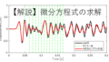
First, we verified that we can estimate the modal characteristics from FRFs with four resonance frequencies. The FRFs used are as follows

By the way, the true resonance frequency ωdr and mode damping ratio ζ are in the table below. You would like to identify this using the RFP method.
| 1st eig. | 2nd eig. | 3rd eig. | 4th eig. | |
| ωdr | 34.73 | 100.00 | 153.21 | 187.94 |
| ζ | 4.00% | 4.00% | 4.00% | 4.00% |
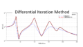
The results of the identification are shown below. I have tried to illustrate it a bit like a stabilization diagram. The identified resonance frequency ωdr and mode damping ratio ζ are shown in the table below.

| 1st eig. | 2nd eig. | 3rd eig. | 4th eig. | |
| ωdr | 34.73 | 100.00 | 153.21 | 187.94 |
| ζ | 4.00% | 4.00% | 4.00% | 4.00% |
You have been able to identify it without error. However, the above result is identified assuming that there are four resonance frequencies in the FRF. In reality, the number of resonance frequencies is unknown, so let’s assume 7 and try the calculation again.

I see that the recalculated FRF results are snoring. In other words, depending on the number of resonance frequencies you want to identify, the results of the modal characteristics will change. (I won’t go into detail, but the results of the modal damping ratio will also be wrong.)
Therefore, it is necessary to set an “appropriate value” for the number of resonance frequencies you want to identify. Alternatively, you can use commercially available mode identification software to calculate the stability of the poles and select only those mode characteristics that are stable. I will explain more about this in the near future.
MATLAB code
executable file
clear all;clc;close all

% freq=30:0.1:40; %Calculated frequency definition
freq=0.1:0.1:40; % calculation frequency definition
df=freq(2) - freq(1);
w=2*pi*freq; %angular frequency
m_vec=ones(1,4);
k_vec=ones(1,4)*10^4;
[M]=eval_Mmatrix(m_vec); %mass matrix
[K]=eval_Kmatrix(k_vec); %stiffness matrix

[V,D]=eig(K,M); % eigenvalue D, eigenvector V
for ii1=1:length(m_vec)
    V(:,ii1)=V(:,ii1)/V(1,ii1); % normalize so that the component of mode vector at excitation point m1 is 1
end
wn=sqrt(diag(D)); % natural angular frequency
fn=wn/(2*pi); % natural frequency

mr=diag(V.'*M*V); %mode mass matrix
kr=diag(V.'*K*V); %mode stiffness matrix
c_cr=2*sqrt(mr.*kr);
modal_dampimg=1*0.04; %modal damping ratio (set to 4% for now)
cr=c_cr*modal_dampimg; %modal damping factor

F=zeros(length(m_vec),1); F(1)=1; %external force vector (all frequency bands are vibrated by 1)
Xj=zeros(length(m_vec),length(freq)); %displacement vector (define vector and allocate memory before calculation)

% % % mode method
ii=1; % excitation points (if there are multiple excitation points, just add a loop for ii=1:kength(F))
for ii1=1:length(m_vec) % response point
    for ii2=1:length(wn)
        Xj(ii1,:)=Xj(ii1,:)+V(ii1,ii2)*V(ii,ii2). /( -mr(ii2). *w.^2 + 1i*cr(ii2)*w +kr(ii2))*F(ii);
% transverse vector = transverse vector +  scalar × scalar . /( scalar × transverse vector + scalar × transverse vector + scalar) × scalar
    end
end

FRF_E=Xj(1,:);


figure
semilogy(w,abs(FRF_E),'k-','linewidth',2)
hold on
xlabel('Angular frequency Hz')
label('Displacement [m]')
xlim([w(1) w(end)])
ylim([min(abs(FRF_E)) max(abs(FRF_E))])
grid on


%%%%%%%%%%%%%%%%%%%%%%%%%%%%%%%%%%%%%%%%%%%%%%%%%%%%%%%%%%%%%%%%%%%%%%%%%%%%%%%%%%
%%%%%%%%%%%%%%%%%%%%%%%%%%%%%%%%%%%%%%%%%RFP
%%%%%%%%%%%%%%%%%%%%%%%%%%%%%%%%%%%%%%%%%%%%%%%%%%%%%%%%%%%%%%%%%%%%%%%%%%%%%%%%%%
N=4;
[FRF_Re,modal_parameter]=Rational_Fraction_Polynomial_Method(FRF_E,freq,N);

semilogy(w,abs(FRF_Re),'r-','linewidth',2)

% % % % I wrote something like a stabilization diagram
Y=logspace(log10(min(abs(FRF_E))),log10(max(abs(FRF_E))),N);
for ii1=1:1:N
    [FRF_Re,modal_parameter]=Rational_Fraction_Polynomial_Method(FRF_E,freq,ii1);
    semilogy(modal_parameter(:,1),Y(ii1)*ones(ii1,1),'bo','linewidth',2)
    semilogy([w(1) w(end)],Y(ii1)*[1 1],'k--','linewidth',1)
end
function file
function [FRF_recalcu,modal_parameter]=Rational_Fraction_Polynomial_Method(FRFdata,freq,N)
% modal_parameter = Modal Parameters [freq,damp,Ci,Oi]:
% fn: Resonance frequency
% damp: Mode damping ratio
% Ci: mode amplitude
% Oi: Mode phase angle


% % % % % % % % % % % % % % % % % initialization
w=2*pi*freq;
[r,c]=size(w);
if r<c
	w=w.';
end
[r,c]=size(FRFdata);
if r<c
	FRFdata=FRFdata.';
end
% % Normalized angular frequency
nom_w=max(w);
w=w./nom_w;
% % % % % % % % % % % % % % % % % % % % % % % % % %

m=2*N-1; %eq(4.60OT)のm
n=2*N;   %eq(4.60OT)のn

%orthogonal function that calculates the orthogonal polynomials
[phi,coeff_A]=Complex_Orthogonal_Polynomials(FRFdata,w,1,m);
[theta,coeff_B]=Complex_Orthogonal_Polynomials(FRFdata,w,2,n);

[r,c]=size(phi);
P=phi(:,1:c);     %eq(4.66OT)のP
[r,c]=size(theta);
Theta=theta(:,1:c); %eq(4.67OT)のθ
T=sparse(diag(FRFdata))*theta(:,1:c-1);
W=FRFdata.*theta(:,c);%式(4.66OT)のW
X=-2*real(P'*T); left-most matrix(1,2) of %Eq.(4.70OT)
G=2*real(P'*W); the right-most vector (1,1) of %Eq.(4.70OT)

D=-inv(eye(size(X))-X.'*X)*X.'*G; %eq(4.72OT)
C=G-X*D;   %eq(4.73OT)
D=[D;1];

%calculation of FRF (alpha)
FRF_recalcu=zeros(length(w),1);
for n=1:length(w),
   numer=sum(C.'.*P(n,:));
   denom=sum(D.'.*Theta(n,:));
   FRF_recalcu(n)=numer/denom;
end

A=coeff_A*C;
[r,c]=size(A);
A=A(r:-1:1).'; %{A} standard numerator polynomial coefficients

B=coeff_B*D;
[r,c]=size(B);
B=B(r:-1:1).'; %{B} standard denominator polynomial coefficients

%calculation of the poles and residues
[R,P,K]=residue(A,B);
[r,c]=size(R);
for n=1:(r/2),
   Residuos(n,1)=R(2*n-1);
   Polos(n,1)=P(2*n-1);
end
[r,c]=size(Residuos);
Residuos=Residuos(r:-1:1)*nom_w; %residues
Polos=Polos(r:-1:1)*nom_w;       %poles
    fn=abs(Polos);                 %Natural frequencies (rad/sec)
    damp=-real(Polos)./abs(Polos);   %Damping ratios

Ai=-2*(real(Residuos).*real(Polos)+imag(Residuos).*imag(Polos));
Bi=2*real(Residuos);
const_modal=complex(Ai,abs(Polos).*Bi);
	Ci=abs(const_modal);             %Magnitude modal constant
	Oi=angle(const_modal).*(180/pi);   %Phase modal constant (degrees)

modal_parameter=[fn, damp, Ci, Oi];    %Modal Parameters


end

% % % % % % % % % % % % % % % % % % % % %

function [P,coeff]=Complex_Orthogonal_Polynomials(FRFdata,w,phitheta,kmax)

if phitheta==1
	q=ones(size(w));         %Weight function for the numerator term (term b)
elseif phitheta==2
	q=(abs(FRFdata)).^2;     %Weight function of the denominator term (term a)
end

R_m1=zeros(size(w));                    %eq(4.1004)
R_0=1/sqrt(2*sum(q)).*ones(size(w));    %eq(4.1005)
Rminus=[R_m1,R_0];                      %polynomials Half Function
coeff=zeros(kmax+1,kmax+2);
coeff(1,2)=1/sqrt(2*sum(q));

%generating orthogonal polynomials matrix and transform matrix
Rplus=[];
R=[Rminus Rplus];
for k=1:kmax,
	Vkm1=2*sum(w.*R(:,k+1).*R(:,k).*q); %IMAC eq(29)
	Sk=w.*R(:,k+1)-Vkm1*R(:,k);         %eq(4.1006)
	Dk=sqrt(2*sum((Sk.^2).*q));         %IMAC eq(31)
	Rplus=[Rplus Sk/Dk];
	coeff(:,k+2)=-Vkm1*coeff(:,k);
	coeff(2:k+1,k+2)=coeff(2:k+1,k+2)+coeff(1:k,k+1);
    coeff(:,k+2)=coeff(:,k+2)/Dk;
    R=[Rminus Rplus];
end

R=R(:,2:kmax+2);         %orthogonal polynomials matrix
coeff=coeff(:,2:kmax+2); %transform matrix

P=R.*i.^(0:kmax);           %eq(4.1003)
jk=i.^(0:kmax);

coeff=(jk'*jk).*coeff;

end
function [M]=eval_Mmatrix(m_vec)

M=diag(m_vec);

end
function [K]=eval_Kmatrix(k_vec)

K=zeros(length(k_vec));
for ii1=1:length(k_vec)
    if ii1==1
        K(ii1,ii1)=k_vec(ii1);
    else
        K(ii1-1:ii1,ii1-1:ii1)=K(ii1-1:ii1,ii1-1:ii1)+[1 -1;-1 1]*k_vec(ii1);
    end
end

end
コメント