Introduction
There are several types of transfer functions (Frequency Response Function (FRF)): H1 estimation, H2 estimation, H3 estimation, and Hv estimation. This article describes H2 estimation.
If you want to see all my lessons in English, please see below.

H2 estimation of FRF
As mentioned in the previous article, H1 estimation is the most common method of estimating the transfer function.
So what about H2 estimation? You may ask.
Frankly, it is not likely to be used at present: ……
First, let us consider an ideal FRF. The ideal FRF G(ω) is as follows.

(入力=input、応答=response)
However, as a practical matter, such an ideal measurement is not possible. In the case of H1 estimation, we considered the case where noise enters the response as shown in the figure below.

(入力=input、応答=response、ノイズ=noise)
In the case of H2 estimation, consider the case of noise at the input as shown in the figure below.

H2 estimation is a method to estimate FRF = (response V)/(input F) in a situation where the input signal contains noise components, as shown in the figure above.
At this point, you may be asking yourself the following question.
Background
If the input is given by generating vibration in a flow such as (signal generator) → (amplifier) → (shaker) as shown in the figure below, the input F can be measured from anywhere.

Specifically, there are three possible ways to do this
(1) Branch the wire connecting the signal generator and amplifier, and measure the input F.
(2) Branch the wire connecting the amplifier to the shaker and measure the input F.
(3) Place an acceleration sensor on the shaker, or install a load cell in the shaker, or measure the input F by using a terminal for reference signal on the shaker itself, etc.
In this case, with ①, the signal is small and may be affected by noise due to the fact that it is branched for measurement. So, it is “not without”.
In the past, there were no power-supplied sensors such as ICPs, etc., so if input F was used as a sensor signal before passing it through an amplifier, etc., would you have used H2 estimation? (I’m guessing quite a bit here.)
Theory of H2 Estimation
The formula for H2 estimation in the textbook itself is very simple. The theoretical formula is based on the following.
$$
H2(ω)= \frac{W_{xx}(ω)}{W_{xf}(ω)}
$$
where Wxf is the Cross Spectral Density Function of X and F and Wxx is the Power Spectral Density Function or Auto Spectral Density Function) of X.
However, the formula for Hz estimation in the textbook is a bit wrong. It is actually the following, where N is the number of times of averaging.
$$
H2(ω)= \frac{\sum_{n=1}^{N} W_{xx}(ω)}{\sum_{n=1}^{N} W_{xf}(ω)}
$$
Or (what I mean below is that it can be obtained from the average of the cross spectral density function and the average of the power spectral density function)
$$
H2(ω)= \frac{\sum_{n=1}^{N} W_{xx}(ω)/N}{\sum_{n=1}^{N} W_{xf}(ω)/N}
$$
Now we will explain why the above equation can reduce noise in the response.
Note that * refers to conjugation. (Note that * does not mean x.)
$$
H2(ω)= \frac{\sum_{n=1}^{N} V(ω)^*V(ω)}{\sum_{n=1}^{N} V(ω)^*(F(ω)+N(ω))}
$$
$$
H2(ω)= \frac{\sum_{n=1}^{N} V(ω)^*V(ω)}{\sum_{n=1}^{N} V(ω)^*F(ω)+V(ω)^*N(ω)}
$$
Since the noise component N is assumed to be uncorrelated noise, it approaches 0 after the averaging process. Therefore, when N is increased and averaged, the uncorrelated noise N converges to 0, resulting in the equation below.
$$
H2(ω)= \frac{\sum_{n=1}^{N} V(ω)^*V(ω)}{\sum_{n=1}^{N} V(ω)^*F(ω)}
$$
Noise can be reduced by the above.
Validation in MATLAB
Result
The results of the analysis are shown first. (100 times average)
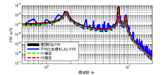
The ideal FRF with no noise component is shown by the black line.
The FRF with noise components and without averaging is represented by the blue line, and
(The H2 estimation result (with averaging) is shown by the red dotted line.
As can be seen from the figure, the error between the ideal FRF and the H2 estimation result is smaller than that of the FRF without averaging.
Note that the noise component is given by ±85% of F as a reference.
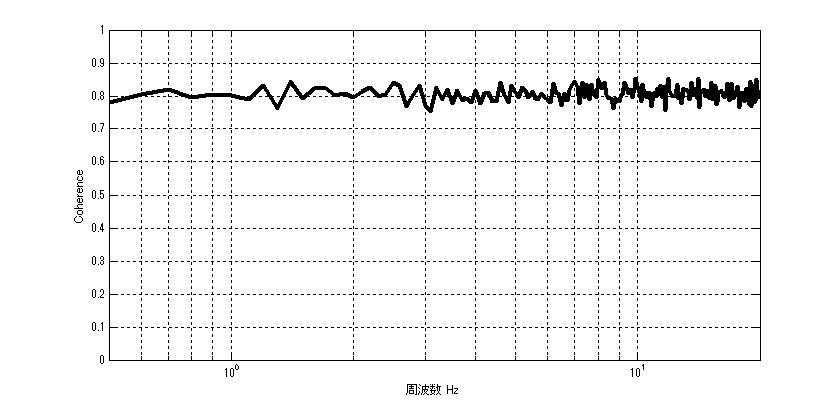
As we will explain in the next section, the coherence function γ^2 can be easily obtained once the H1 and H2 estimation can be programmed.
$$
γ^2_{fx}(ω)= \frac{H1}{H2}
$$
The coherence function in this study is shown in the figure below.
MATLAB code
Executable file
clear all
close all
% % % % 初期設定
freq=0.5:0.1:20;
m_vec=[1 1 1 1];
[M]=eval_Mmatrix(m_vec);
k_vec=[1 1 1 1]*10^3;
[K]=eval_Kmatrix(k_vec);
C=zeros(length(k_vec));
F=zeros(length(m_vec),length(freq));
F(1,:)=ones(1,length(freq));

% % % % 変位X(ノイズなし)
X=eval_direct_x_2ndedition(M,K,C,F,freq);
% % % % 理想的なFRF
FRF_ideal_x3_f1=X(3,:)./F(1,:);

N=100; %平均化回数 100回
res=zeros(N,length(freq));
ref=zeros(N,length(freq));
for ii1=1:N
    res(ii1,:)=X(3,:);
    ref(ii1,:)=F(1,:)+( rand(1,length(freq)) - 0.5 )*2*0.85; % Fを基準として±85%のノイズを加える
end

[h1] = H1(ref,res,freq);
[h2] = H2(ref,res,freq);

figure(1)
loglog(freq,abs(FRF_ideal_x3_f1),'k','linewidth',7)
hold on
loglog(freq,abs(res(1,:)./ref(1,:)),'b','linewidth',3)
loglog(freq,abs(h1),'g--','linewidth',3)
loglog(freq,abs(h2),'r--','linewidth',3)
hold off
grid on
legend('理想的なFRF','平均化処理をしないFRF','H1推定','H2推定')
xlim([freq(1) freq(end)])
xlabel('周波数 Hz');ylabel('FRF m/N');

figure
semilogx(freq,h1./h2,'k','linewidth',3)
xlabel('周波数 Hz');ylabel('Coherence');
grid on
ylim([0 1])
xlim([freq(1) freq(end)])
function file
function [K]=eval_Kmatrix(k_vec)
K=zeros(length(k_vec));
for ii1=1:length(k_vec)
    if ii1==1 K(ii1,ii1)=k_vec(ii1);
    else
        K(ii1-1:ii1,ii1-1:ii1)=K(ii1-1:ii1,ii1-1:ii1)+[1 -1;-1 1]*k_vec(ii1);
    end
end

end
function [M]=eval_Mmatrix(m_vec)
M=diag(m_vec);
end
function x=eval_direct_x_2ndedition(M,K,C,F,freq)
% % 2021.05.28 Fを修正
x=zeros(size(F,1),length(freq));
j=sqrt(-1);
for ii1=1:1:length(freq)
    w=2*pi*freq(ii1);
    x(:,ii1)=inv(K+j*w*C-w^2*M)*F(:,ii1);
end

end
function [Wff]=PowerSpectralDensity(F,freq)

if size(F,1)==length(freq)
    F=F.';
end

Wff=conj(F).*F;


end
function [Wfx]=CrossSpectralDensity(F,X,freq)

if size(F,1)==length(freq)
    F=F.';
end
if size(X,1)==length(freq)
    X=X.';
end


Wfx=conj(F).*X;


end
function [h1] = H1(ref,res,freq)

% h1=zeros(1,freq);

[Wfx]=CrossSpectralDensity(ref,res,freq);
[Wff]=PowerSpectralDensity(ref,freq);

h1=mean(Wfx,1)./mean(Wff,1);

end
function [h2] = H2(ref,res,freq)

% h1=zeros(1,freq);

[Wxf]=CrossSpectralDensity(res,ref,freq);
[Wxx]=PowerSpectralDensity(res,freq);

h2=mean(Wxx,1)./mean(Wxf,1);

end
コメント