Introduction
When identifying resonant frequencies and vibration modes, we look at the FRF peaks and think “I wonder if this is the resonant frequency”.
However, it is not always the case that (peak FRF frequency) = (resonant frequency).
As those who have experienced hammering or excitation tests, the lower-order FRF peak value is easy to determine as the resonance frequency, but the higher-order FRF peak value is not.
The higher-order FRF peak values are densely concentrated in a narrow band, making it difficult to determine whether they are resonance frequencies, just peak values, or noise.
It is also impossible to determine the overlapping roots (when two resonance frequencies exist at the same frequency).
This article explains how to identify the resonance frequency using the mode indicator function.
The following link is a summary to a description of vibration theory in English, if you are interested.

I’ve also developed my own curve fitting software.
If you’re interested, feel free to download it from the link below and give it a try.
👉 Free Download
Modal Indicator Functions
Do you know Modal Indicator Functions(MIFs)?
There are several types of modal indicator functions: CMIF, MMIF, and RMIF.
Here, CMIF (Complex Modal Indicator Functions) are introduced.
Ewin’s book “Modal Testing” provides the explanation of modal indicator functions.
MMIF(Multivariate Modal Indicator Functions)
The following are the theoretical equations for MMIF. The theoretical equation is based on the following reference.
MMIF takes a value between 0 and 1, and is characterized by the fact that it is close to 0 at frequencies where resonance frequencies exist. Therefore, it is easy to determine the resonance frequency.
MMIF is the eigenvalue β of the following equation.
where H_Real is the real part of the transfer function matrix H(ω) and H_Imag is the imaginary part of the transfer function matrix H(ω). ω is omitted because of the length of the equation. (“Modal Testing” by Ewin)
$$
β([H_{Real}]^T[H_{Real}]+[H_{Imag}]^T[H_{Imag}]){F}=([H_{Imag}]^T[H_{Imag}]){F}
$$
By the way, if I remember correctly, I think the upper formula was wrong. I think the correct formula was the lower one. (I verified this when I was a student, but I would like to re-verify it again. I’m not sure, so I grayed out the text.)
I made MATLAB code of MMIF following eq.
$$
β([H_{Real}]^T[H_{Real}]+[H_{Imag}]^T[H_{Imag}]){F}=([H_{Real}]^T[H_{Real}]){F}
$$
Validation in MATLAB
Verification by executable file
The MMIF results for 2-point excitation and 4-point response are shown in the figure below.
From the figure, it can be seen that the resonance frequency and the peak value of MMIF coincide.
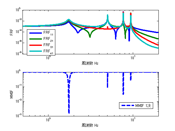
Figure 1 Result of Executable File
Incidentally, commercially available experimental mode analysis software often displays MMIF on the resonance frequency determination screen. That is how trustworthy and intuitively easy to understand it is. However, software users often use MMIF without understanding what it means.
I recommend using both MMIF and CMIF to determine and select resonance frequencies while checking for overlapping roots. The reason is that the habit of checking both MMIF and CMIF makes it easier to identify resonance frequencies when analyzing high frequencies, even if the resonance frequencies are dense.
MATLAB code
Executable File
clear all
close all
% % % % 初期設定
freq=0.5:0.01:20;
m_vec=[1 1 1 1];
[M]=eval_Mmatrix(m_vec);
k_vec=[1 1 1 1]*10^3;
[K]=eval_Kmatrix(k_vec);
C=ones(length(k_vec))*0.2;
F1=zeros(length(m_vec),length(freq));
F1(1,:)=ones(1,length(freq));
F2=zeros(length(m_vec),length(freq));
F2(2,:)=ones(1,length(freq));
% % % % 変位X(ノイズなし)
X1=eval_direct_x_2ndedition(M,K,C,F1,freq);
X2=eval_direct_x_2ndedition(M,K,C,F2,freq);
% % % % 理想的なFRF
FRF_x4_f1=X1(4,:)./F1(1,:);
FRF_x3_f1=X1(3,:)./F1(1,:);
FRF_x2_f1=X1(2,:)./F1(1,:);
FRF_x1_f1=X1(1,:)./F1(1,:);

FRF_x4_f2=X2(4,:)./F2(2,:);
FRF_x3_f2=X2(3,:)./F2(2,:);
FRF_x2_f2=X2(2,:)./F2(2,:);
FRF_x1_f2=X2(1,:)./F2(2,:);


inputN=2;
MMIF=zeros(1,length(freq));

for ii1=1:length(freq)
    H=[ FRF_x1_f1(ii1) FRF_x1_f2(ii1)
        FRF_x2_f1(ii1) FRF_x2_f2(ii1)
        FRF_x3_f1(ii1) FRF_x3_f2(ii1)
        FRF_x4_f1(ii1) FRF_x4_f2(ii1)
        ];
    HH=pinv(real(H).'*real(H)+imag(H).'*imag(H))*real(H).'*real(H);
    [V,D]=eig(HH);
    MMIF(1,ii1)=min(diag(D));

end

figure
subplot(211)
loglog(freq,abs([FRF_x1_f1;FRF_x2_f1;FRF_x3_f1;FRF_x4_f1]),'linewidth',3)
xlim([freq(1) freq(end)])
xlabel('周波数 Hz');ylabel('FRF');
legend('FRF_1_1','FRF_2_1','FRF_3_1','FRF_4_1')
subplot(212)
loglog(freq,MMIF,'--','linewidth',3)
xlim([freq(1) freq(end)])
xlabel('周波数 Hz');ylabel('MMIF');
legend('MMIF')
function file
function [K]=eval_Kmatrix(k_vec)
K=zeros(length(k_vec));
for ii1=1:length(k_vec)
    if ii1==1 K(ii1,ii1)=k_vec(ii1);
    else
        K(ii1-1:ii1,ii1-1:ii1)=K(ii1-1:ii1,ii1-1:ii1)+[1 -1;-1 1]*k_vec(ii1);
    end
end

end
function [M]=eval_Mmatrix(m_vec)
M=diag(m_vec);
end
function x=eval_direct_x_2ndedition(M,K,C,F,freq)
% % 2021.05.28 Fを修正
x=zeros(size(F,1),length(freq));
j=sqrt(-1);
for ii1=1:1:length(freq)
    w=2*pi*freq(ii1);
    x(:,ii1)=inv(K+j*w*C-w^2*M)*F(:,ii1);
end

end
コメント