
Introduction
I am re-reviewing the bible-like book “Introduction to Modal Analysis,” which every Japanese vibration engineer has read at least once.
I would like to explain what I have learned in the re-review, showing the MATLAB code. This time, we will review from section 6.3.2, “Prony Method,” p. 367. The “poly-reference method” is an extension of the Prony method to the multipoint reference method. (also called “Vold’s method” since it was drafted by Vold).
The mode identification method with a function called modalfit, introduced in the Signal Processing Toolbox of MATLAB2017a, can also be solved by the “Prony method”. Please refer to MathWorks’ website for details. Incidentally, “FitMethod”=”lsce”, the default mode identification method of modalfit, is explained as the Prony method.
The following link is a summary to a description of vibration theory in English, if you are interested.

I’ve also developed my own curve fitting software.
If you’re interested, feel free to download it from the link below and give it a try.
👉 Free Download
6.3.2 Prony’s method
In previous articles, I have explained that FRFs and vibration shapes can be expressed as a superposition of modal characteristics (resonant frequencies & vibration modes, etc.). It is the concept of modal analysis. And extracting mode characteristics from FRF is called mode identification or curve fitteing.
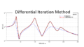
The mode circle fitting (curve fitting) and half-width method were applicable only when the adjacent resonance frequencies are far enough apart, as in the red frequency band in Figure 1, and the system can be regarded as a one-degree-of-freedom system.
 Figure 1 FRF
On the other hand, Prony’s method is a mode identification method for multi-degree-of-freedom systems. In other words, it is a method that can extract the mode characteristics of each resonance frequency even if it contains multiple resonance frequencies, such as the 0 to 100 Hz data in Figure 1.
From here, the explanation becomes a bit more technical.
Prony’s method is a method to estimate modal characteristics from impulse response data. Although it is possible to use time history data of the response of impact excitation with an impact hammer, etc., it is known that the signal-to-noise ratio is generally bad, and in many cases, data obtained by IFFT of FRF averaged over the number of measurements and then the data, converted back to impulse response, is used as input for the Prony’s method.
Since the impulse response can be expressed as a superposition of mode characteristics, it can be expressed as in Equation (6.52).
$$
h(t)=\sum_{r=1}^{N} a_{r}(je^{λ_r t} – je^{λ_r^* t} ) \tag{6.52}
$$
where λr is the eigenvalue, ωdr is the damped natural angular frequency, and σr is the modal damping factor, detailed in the equation below.
$$
a_r=\frac{ Ω_r^2 }{2ω_{dr}K_r}, λ_r=-σ_r + jω_{dr}, λ_r^*=-σ_r – jω_{dr} \tag{6.51}
$$
However, rather than the above equation, it is better to just remember that ar is the residu, λr is the eigenvalue, ωdr is the damped natural angular frequency, and σr is the modal damping rate.
Again, mode identification means finding the distn ar and eigenvalue λr.
There are various methods for mode identification, but they differ only in their approach to finding the abscissa ar and eigenvalue λr.
Since the data are discretized, equation (6.53) can be expressed in a discretized form for time t as in equation (6.54). Note that i is the data id. It is assumed that only n (n<N) of N are to be identified, rather than all N, the number of all resonance frequencies.
$$
h(iΔt)=\sum_{r=1}^{n} a_{r}(e^{λ_r iΔt} – e^{λ_r^* iΔt} ) \tag{6.52}
$$
Here, since the character expression is complicated, it is replaced by the following for simplicity.
$$
x_r=e^{λ_r Δt}, x_r^*=e^{λ_r^* Δt} \tag{6.55}
$$
Then it can be expressed as in equation (6.56).
$$
h(iΔt)=\sum_{r=1}^{n} a_{r}(x_r^i + x_r^{i*} )=\sum_{r=1}^{n} real( 2a_{r}(x_r^i ) )=\sum_{r=1}^{2n} a_{r}(x_r^i ) \tag{6.56}
$$
I think some of you may not understand the equation expansion of equation (6.56). Originally, the expansion was based on the assumption that n resonance frequencies are to be identified, but since it is more coherent to identify 2n resonance frequencies, the number of resonance frequencies is 2n.
You can manage to get to this point.
Equation (6.56) is just a repeated transformation of the equation, and as it is, we can’t extract the distnumber ar and eigenvalue λr, can we?
For now, let’s consider equation (6.56) in a simplified form, with n=2 and i=0,1,2,3,4.
\(
h(0)=a_1 x_1^0 + a_2 x_2^0 + a_3 x_3^0 + a_4 x_4^0
\\
h(1)=a_1 x_1^1 + a_2 x_2^1+ a_3 x_3^1 + a_4 x_4^1
\\
h(2)=a_1 x_1^2 + a_2 x_2^2 + a_3 x_3^2 + a_4 x_4^2
\\
h(3)=a_1 x_1^3 + a_2 x_2^3 + a_3 x_3^3 + a_4 x_4^3
\\
h(4)=a_1 x_1^4 + a_2 x_2^4 + a_3 x_3^4 + a_4 x_4^4
\)
$$
\tag{6.56.0}
$$
In this situation, we can’t extract the abstention number ar and eigenvalue λr, can we?
So, consider the following.
$$
(x-x_1)(x-x_1^*)(x-x_2)(x-x_2^*) =0 \tag{6.57.3}
$$
Since it is difficult to calculate by hand, we replace it with the following so that it can be solved by Maxima.
$$
(x-a1)(x-c1)(x-a2)(x-c2) =0
$$
Expanding the above equation, we get
\(
x^4 \\ +(-c2-c1-a2-a1)x^3 \\ +(c1*c2+a2*c2+a1*c2+a2*c1+a1*c1+a1*a2)x^2 \\ +(-a2*c1*c2-a1*c1*c2-a1*a2*c2-a1*a2*c1)x \\ +a1*a2*c1*c2 =0
\)
$$
\tag{6.57.0}
$$
Replace the above with the following. Note that b4=1 here.
\(
b_4 x^4 \\ +b_3 x^3 \\ +b_2 x^2 \\ +b_1 x^1 \\ +b_0 x^0 =0
\)
$$
\tag{6.57.1}
$$
Equation (6.57.1) is a generalization of equation (6.57).
$$
\sum_{i=0}^{2n}b_i x^i =0 \tag{6.57}
$$
Now we will consider how to extract the abstention number ar and the eigenvalue λr, comparing equations (6.56.0) and (6.57.1). For now, let us multiply both sides of equation (6.56.0) by bi.
\(
b_0 h(0)=b_0 (a_1 x_1^0 + a_2 x_2^0 + a_3 x_3^0 + a_4 x_4^0)
\\
b_1 h(1)=b_1 (a_1 x_1^1 + a_2 x_2^1+ a_3 x_3^1 + a_4 x_4^1)
\\
b_2 h(2)=b_2 (a_1 x_1^2 + a_2 x_2^2 + a_3 x_3^2 + a_4 x_4^2)
\\
b_3 h(3)=b_3 (a_1 x_1^3 + a_2 x_2^3 + a_3 x_3^3 + a_4 x_4^3)
\\
b_4 h(4)=b_4 (a_1 x_1^4 + a_2 x_2^4 + a_3 x_3^4 + a_4 x_4^4)
\)
$$
\tag{6.60.0}
$$
All of equation (6.60.0) can be added together and summarized as follows
$$
\sum_{i=0}^{2*2}b_i h(i) = a_1 \sum_{i=0}^{2*2}b_i x_1^i +a_2 \sum_{i=0}^{2*2}b_i x_1^i +a_3 \sum_{i=0}^{2*2}b_i x_3^i +a_4 \sum_{i=0}^{2*2}b_i x_4^i \tag{6.60.1}
$$
rom equation (6.57), equation (6.60) becomes equation (6.61.0).
$$
\sum_{i=0}^{2*2}b_i h(i) = 0 \tag{6.61.0}
$$
A slight variant of equation (6.61.0)
$$
b_4 h(4) + \sum_{i=0}^{2*2-1}b_i h(i) = 0 \tag{6.61.1}
$$
Here, b4=1, so the equation below holds.
$$
-h(4) = \sum_{i=0}^{2*2-1}b_i h(i) \tag{6.62.0}
$$
In the Introduction to Modal Analysis, there is a generalized explanation of the above. However, if you are a gory mode identification enthusiast like me, I would like to add a supplemental explanation that is a little different.
For example, suppose that the impulse response is as shown in Figure 2 with i = 0 to 2n-1 and the time history data is for 0.1 second.
Assuming a time resolution of 0.0001, the way to take 0.1 second of the impulse response is
0 to 0.1 second, or
0.0001 to 1.0001 seconds is also fine.
 図2 インパルス応答
Therefore, a known method is to calculate b such that the error is minimized using a large number of 0.1 second data. Specifically, we solve as in Equations (6.62.1)-(6.62.3).
\(
\left(
\begin{array}{ccc}
h(0) & \ldots & h(2n-1) \\
\vdots & \ddots & \vdots \\
h(2n-1) & \ldots & h(4n-2)
\end{array}
\right)
\left(
\begin{array}{c}
b_0 \\
\vdots \\
b_{2n-1}
\end{array}
\right)=
\left(
\begin{array}{c}
h(2n) \\
\vdots \\
h(4n-1)
\end{array}
\right) \tag{6.62.1}
\)
Equation (6.62.2) is a simplified version of Eq(6.62.1).
$$
Hb=y \tag{6.62.2}
$$
Considering that y contains an error, equation (6.62.3) is the solution of b by the least-squares method.
$$
b=(H^tH)^{-1} H^t y \tag{6.62.2}
$$
Now you have obtained b.
Once b is obtained, solving the algebraic equation in Eq. (6.57) yields xr in Eq. (6.55).
From xr, we obtain the damped angular resonance frequency ωdr and the modal damping factor σr as in the equation below.
$$
σ_r=-\frac{In|x_r|}{Δt} \tag{6.100.1}
$$
$$
ω_{dr}=\frac{1}{Δt}atan(\frac{imag(x_r)}{real(x_r)}) \tag{6.100.2}
$$
Theoretical formulas up to the above may be found in modal analysis handbooks and other sources of modal identification.
However, the above theoretical equations alone cannot identify the mode characteristics. Rather, the Prony method requires the identification of a larger number of resonance frequencies. For example, a waveform with only two resonance frequencies excited is assumed to have 50 resonance frequencies by the Prony method to estimate the mode characteristics.
Therefore, it is necessary to extract the two that seem to be correct from the estimated 50. In some cases, the 50 may not have been estimated correctly in the first place. We need to make these judgments, but the indicators for making these judgments are not described in any commercially available reference book.
I would like to explain the above issues using examples.
Example of MATLAB
Solution from eq(6.52) to eq(6.62.2)
Let us now solve the example problem in MATLAB.
Let us find the modal characteristics from the impulse response waveforms with resonance frequencies of 10Hz and 50Hz as shown in Figure 3. Note that the modal damping ratios are 5%@10Hz and 1%@50Hz.
 Figure 3 Impulse response
Now, let’s make the waveform shown in Figure 4, and the MATLAB program will look like the following.
clear all;clc;close all;

j=sqrt(-1);
time=0:0.0001:1;

% % Example of time response vector X
freq1=10; omega1=freq1*2*pi;
freq2=50; omega2=freq2*2*pi;
zeta1=0.05; sgm1=zeta1*omega1;
zeta2=0.01; sgm2=zeta2*omega2;
phi1=0; phi2=0;
X=exp(-zeta1*omega1*time).*sin(omega1*time+phi1)......
 +exp(-zeta2*omega2*time).*sin(omega2*time+phi2);

figure
plot(time,X)
xlabel('Time [s]')
ylabel('Ampli [mm]')
Now that we have created the impulse response waveform, let’s program it up to the Prony method equation (6.62.2). By the way, the program is as follows.
% Number of resonance frequencies N to be sought (the trick is to set a larger number for now)
% N-1 to be sought
N=10; n=N/2;

% % eq(6.62.1) H
H=zeros(2*n);
for ii1=1:2*n
    H(ii1,:)=X(ii1:(ii1+2*n-1)).';
end

% % Right side of Eq. (6.62.1) (y-vector in Eq. (6.62.2))
y=-X(2*n+1:n*4).';


% % eq(6.62.2)
b=(H.'*H)(H'*y);
You have found b in equation (6.62.2).
From b, you can find the mode characteristic by finding x that satisfies equation (6.57).
Estimation of mode properties using “roots” MATLAB function (doesn’t work)
Now, here comes the hard part. How do we solve equation (6.57)?
MATLAB has a function “roots” to find the roots of polynomials.
Let’s try it here (as I mentioned earlier, this method does not work)
r = roots(b.'); %apply roots function to eq(6.57.3)......
% figure
% plot(real(r),imag(r),'.')
% axis equal
% grid on

omega_prony = angle(r)/time(2); %eq(6.100.2)
fn_prony = omega_prony/(2*pi);
sgm_prony = -log(abs(r))/time(2); %eq(6.100.1)
zeta_prony = sgm_prony./omega_prony;
The resonant frequency and mode damping ratio obtained by the above program are as follows
 Figure 4 Obtained mode characteristics (resonant frequency and mode attenuation ratio)
Theoretical values are fn=10, 50; zeta=0.05, 0.01.
Since the Prony method requires a larger order to be identified, this example estimates 9 resonant frequencies and mode damping ratios, but I do not see any combination that matches the theoretical values.
If we increase the number of resonant frequencies to be estimated, we may find a combination that matches the theoretical value. (It is very likely that they will.) However, it is difficult to select the most plausible combination from a huge number of combinations of resonant frequencies and mode damping ratios. To begin with, we are estimating without prior information on how many resonance frequencies are included in the impulse response waveform, so we would like to have a criterion for selecting a combination.
This is the difficult part of mode identification. (This is where mode identification maniacs get hooked.)
Most of the theory of mode identification does not work well even if you program the theoretical equation as it is written in a paper or a reference book. In order to create a program, it is necessary to unravel the information hidden behind the theoretical equation.
Proposed Method
Again, once b is obtained, it is considered possible to extract the modal characteristics by finding xi that satisfies the equality in equation (6.57).
$$
\sum_{i=0}^{2n}b_i x^i =0 \tag{6.57}
$$
So what value is xi likely to be?
To begin with, xi was the following, right? (xr and xi are different orders of resonance, r-order or i-order.)
$$
x_r=e^{λ_r Δt} \tag{6.55}
$$
Also, λr is the following.
$$
λ_r=-σ_r + jω_{dr} \tag{6.51}
$$
Thus,
$$
x_r=e^{(-σ_r + jω_{dr})Δt}=e^{(-ω_{dr}ζ + jω_{dr})Δt}
$$
What is the realistic range of modal attenuation ratio ζ?
Empirically, it should be as follows
0<ζ<0.1
The next thing to consider is the range of resonant frequencies we want to find.
Since this is an example problem, we know the answer to the resonant frequency of the impulse response waveform.
However, (unless you have checked the spectrum in advance and have an estimate of the resonance frequency), you would not normally perform mode identification with the resonance frequency known.
When performing mode identification, the key point is to specify the frequency range you want to find and to limit the frequency range to be sought using the Prony method.
For example, in this example, let’s say you want to find resonance frequencies below 100 Hz. (Assume that you are solving without knowing the number of resonance frequencies in the impulse response waveform or the resonance frequencies themselves.)
In other words, the range where resonant frequencies are likely to exist is as follows.
0<fn<100
0<ωn<2*pi*100
Therefore, the range of ζ and ωn determines the range that x_r can also take.
In MATLAB, x (x_r is defined as x for search) is defined as follows.
Here, x is made to correspond to a change in ζ in the row direction and a change in ωn in the column direction.
We then find the left-hand side of Eq. (6.57).
fn_min=0;
fn_max=100;
zeta_min=0.00001; %モード減衰比が0になることはないので、限りなく小さくしておく
zeta_max=0.1;
dt=time(2);

fn_range=fn_min:0.5:fn_max;
wn_range=2*pi*fn_range;
zeta_range=linspace(zeta_min,zeta_max,1000);

x=exp((-zeta_range.'+j)*wn_range*dt);

Eq_6_57=1*x.^(2*n); %b_2n*x.^(2*n)
for ii1=1:2*n
    Eq_6_57=Eq_6_57+b(ii1)*x.^(ii1-1); %式(6.57)
end
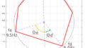
If we can find x such that Eq_6_57, the left side of Eq. (6.57), becomes 0, i.e., a minimum value, we can extract the modal characteristics that are consistent with the theoretical values.
The minimum value is considered to be obtained as follows.
% Determination and search for poles
surf_Eq_6_57 = abs(Eq_6_57);
surf_pole_logical = islocalmin(surf_Eq_6_57,1) & islocalmin(surf_Eq_6_57,2); % Finding the smallest point on a plane (matrix)

xr = x(surf_pole_logical); %pole

omega_prony = angle(xr)/dt; %eq(6.100.2)
fn_prony=omega_ans/(2*pi);
sgm_prony = -log(abs(xr))/dt; %eq(6.100.1)
zeta_prony = sgm_prony./omega_prony;
The results are as follows. The theoretical value is firmly obtained.
 図5 提案手法の結果
MATLAB code (full ver.)
Check that the results of the resonance frequency and mode damping ratio estimation are correct when the amplitudes A1 and A2 are changed, etc.
clear all;clc;close all;

j=sqrt(-1);
time=0:0.0001:1;
dt=time(2);

% Number of resonance frequencies N to be sought (the trick is to set a larger number for now)
% N-1 to be sought
N=100; n=N/2;

% % Example of time response vector X
A1=1; freq1=10; omega1=freq1*2*pi;
A2=2; freq2=50; omega2=freq2*2*pi;
zeta1=0.05; sgm1=zeta1*omega1;
zeta2=0.01; sgm2=zeta2*omega2;
phi1=0; phi2=0;
X=A1*exp(-zeta1*omega1*time).*sin(omega1*time+phi1)......
 +A2*exp(-zeta2*omega2*time).*sin(omega2*time+phi2);

figure
plot(time,X)
xlabel('Time [s]')
ylabel('Ampli [mm]')

% % eq(6.62.1) H
H=zeros(2*n);
for ii1=1:2*n
    H(ii1,:)=X(ii1:(ii1+2*n-1)).';
end

% % Right side of eq.(6.62.1) (equation (6.62.2) y-vector)
y=-X(2*n+1:n*4).';

% % eq(6.62.2)
b=(H.'*H)(H'*y);


fn_min=0;
fn_max=100;
zeta_min=0.00001; % Keep the modal damping ratio as small as possible since it will never be zero.
zeta_max=0.1;

fn_range=fn_min:0.5:fn_max;
wn_range=2*pi*fn_range;
zeta_range=linspace(zeta_min,zeta_max,1000);

x=exp((-zeta_range.'+j)*wn_range*dt);

Eq_6_57=1*x.^(2*n); %b_2n*x.^(2*n)
for ii1=1:2*n
    Eq_6_57=Eq_6_57+b(ii1)*x.^(ii1-1); %eq(6.57)
end

% Determination and search for poles
surf_Eq_6_57 = abs(Eq_6_57);
surf_pole_logical = islocalmin(surf_Eq_6_57,1) & islocalmin(surf_Eq_6_57,2); % 平面上(行列上)の極小点を探す

xr = x(surf_pole_logical); %pole

omega_prony = angle(xr)/dt; %eq(6.100.2)
fn_prony=omega_prony/(2*pi)
sgm_prony = -log(abs(xr))/dt; %eq(6.100.1)
zeta_prony = sgm_prony./omega_prony
コメント