Introduction
In the past, I have introduced several types of transfer functions (Frequency Response Function (FRF)): H1 estimation, H2 estimation, H3 estimation, and Hv estimation.
This article describes the FRF coherence function. The coherence is an indicator of how reliable the FRF is.
If you want to see all my lessons in English, please see below.

Coherence function
Some of you who are or have been studying vibration engineering may have tried to program a coherence function and have not been successful.
There are two complicated aspects of coherence functions.
1st point:Why it’s complicated to understand
The first complication is that there are numerous formulas for coherence functions in textbooks and reference books. (However, they are the same when expanded? Shouldn’t they?)
For example, in “Introduction to Modal Analysis,” the coherence function is expressed in five equations. (The figure below is for reference.)
スポンサーリンク
$$
γ^2_{fx}= \frac{W_{vv}}{W_{xx}}=\frac{\bar{V}V}{W_{xx}}=\frac{\bar{F H1}F H1}{W_{xx}}=\frac{\bar{H1}FF H1}{W_{xx}}=\frac{\bar{H1}W_{ff} H1}{W_{xx}}
$$
$$
γ^2_{fx}= \frac{(\bar{W_{fx}} / \bar{W_{ff}})W_{ff}(W_{fx} / W_{ff})}{W_{xx}}=\frac{\bar{W_{fx}} W_{ff}W_{fx}}{W_{xx}\bar{W_{ff}} W_{ff}}
$$
$$
γ^2_{fx}= \frac{\bar{W_{fx}}W_{fx}}{W_{ff}W_{xx}}= \frac{<W_{fx}W_{fx}>}{W_{ff}W_{xx}}
$$
$$
γ^2_{fx}= \frac{\|W_{fx}\|^2}{\|F\|^2\|X\|^2}
$$
$$
γ^2_{fx}= \frac{\|W_{fx}\|^2}{\|F\|^2\|X\|^2}
$$
$$
γ^2_{fx}(ω)= \frac{H1}{H2}
$$
スポンサーリンク
2nd point:Why it’s complicated to understand
The second complication is that it is unclear where the averaging should be done.
For example, in the equation below, it is unclear whether Wfx, etc., should be averaged by itself, or whether each denominator and numerator should be averaged, or whether the following equation should be obtained for the number of averaging times and then the averaging process should be performed.
$$
γ^2_{fx}=\frac{\bar{W_{fx}} W_{ff}W_{fx}}{W_{xx}\bar{W_{ff}} W_{ff}}
$$
Recommendation
In the equation below, the coherence function can be easily obtained as long as H1 and H2 are well obtained.
$$
γ^2_{fx}(ω)= \frac{H1}{H2}
$$
If you do not know the H1 or H2 estimates, please refer to the following.
Validation in MATLAB
Analysis Results
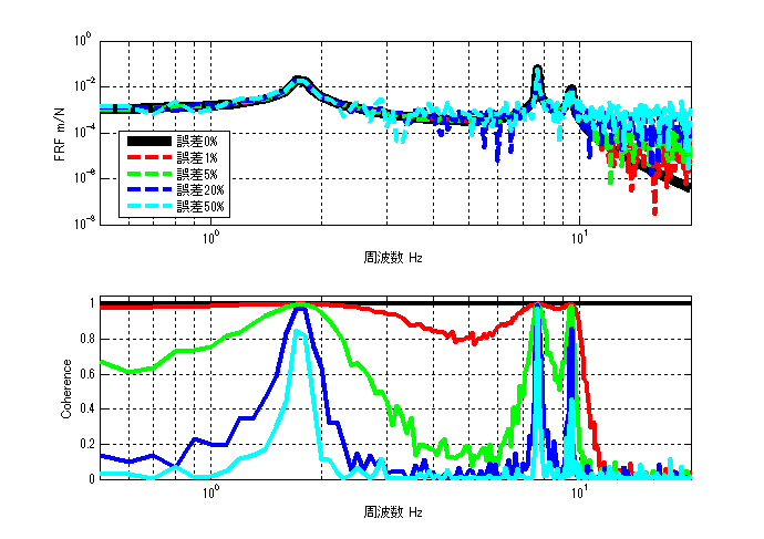
The results of the analysis are shown first. (100 times average)
With no error, the coherence function is 1, and as the error increases, the coherence function approaches 0.
Also, since the response is higher at resonant frequencies, the signal-to-noise ratio (signal-to-noise ratio) improves, which means that the coherence function is closer to 1.
MATLAB Code
Executable file
clear all
close all
% % % % 初期設定
freq=0.5:0.1:20;
m_vec=[1 1 1 1];
[M]=eval_Mmatrix(m_vec);
k_vec=[1 1 1 1]*10^3;
[K]=eval_Kmatrix(k_vec);
C=zeros(length(k_vec));
F=zeros(length(m_vec),length(freq));
F(1,:)=ones(1,length(freq));

% % % % 変位X(ノイズなし)
X=eval_direct_x_2ndedition(M,K,C,F,freq);
% % % % 理想的なFRF
FRF_ideal_x3_f1=X(3,:)./F(1,:);

N=100; %平均化回数 100回
res=zeros(N,length(freq));
res2=zeros(N,length(freq));
res3=zeros(N,length(freq));
res4=zeros(N,length(freq));
ref=zeros(N,length(freq));
for ii1=1:N
    res(ii1,:)=X(3,:)+( rand(1,length(freq)) - 0.5 )*max(abs(X(3,:)))*0.01; % 最大変位Xを基準として1%のノイズを加える
    res2(ii1,:)=X(3,:)+( rand(1,length(freq)) - 0.5 )*max(abs(X(3,:)))*0.05;
    res3(ii1,:)=X(3,:)+( rand(1,length(freq)) - 0.5 )*max(abs(X(3,:)))*0.20;
    res4(ii1,:)=X(3,:)+( rand(1,length(freq)) - 0.5 )*max(abs(X(3,:)))*0.50;
    ref(ii1,:)=F(1,:);
end

[h1_1] = FRF(ref,res,freq,'H1');
[h1_2] = FRF(ref,res2,freq,'H1');
[h1_3] = FRF(ref,res3,freq,'H1');
[h1_4] = FRF(ref,res4,freq,'H1');
[r2_1] = Coherence(ref,res,freq);
[r2_2] = Coherence(ref,res2,freq);
[r2_3] = Coherence(ref,res3,freq);
[r2_4] = Coherence(ref,res4,freq);
[r2_0] = Coherence(ref(1,:),X(3,:),freq);

figure(1)
subplot(211)
loglog(freq,abs(FRF_ideal_x3_f1),'k','linewidth',7)
hold on
loglog(freq,abs(h1_1),'r--','linewidth',3)
loglog(freq,abs(h1_2),'g--','linewidth',3)
loglog(freq,abs(h1_3),'b--','linewidth',3)
loglog(freq,abs(h1_4),'c--','linewidth',3)
hold off
grid on
legend('誤差0%','誤差1%','誤差5%','誤差20%','誤差50%')
xlim([freq(1) freq(end)])
xlabel('周波数 Hz');ylabel('FRF m/N');

subplot(212)
semilogx(freq,r2_0,'k','linewidth',3)
hold on
semilogx(freq,r2_1,'r','linewidth',3)
semilogx(freq,r2_2,'g','linewidth',3)
semilogx(freq,r2_3,'b','linewidth',3)
semilogx(freq,r2_4,'c','linewidth',3)

xlabel('周波数 Hz');ylabel('Coherence');
grid on
ylim([0 1.05])
xlim([freq(1) freq(end)])
function file
function [frf] = FRF(ref,res,freq,FRFtype)


switch FRFtype
    case 'H1'
        [frf] = H1(ref,res,freq);
    case 'H2'
        [frf] = H2(ref,res,freq);
    case 'H3'
        [frf] = H3(ref,res,freq);
    case 'Hv'
        [frf] = Hv(ref,res,freq);
end

end
function [h1] = H1(ref,res,freq)

% h1=zeros(1,freq);

[Wfx]=CrossSpectralDensity(ref,res,freq);
[Wff]=PowerSpectralDensity(ref,freq);

h1=mean(Wfx,1)./mean(Wff,1);

end
function [h2] = H2(ref,res,freq)

% h1=zeros(1,freq);

[Wxf]=CrossSpectralDensity(res,ref,freq);
[Wxx]=PowerSpectralDensity(res,freq);

h2=mean(Wxx,1)./mean(Wxf,1);

end
function [h3] = H3(ref,res,freq)

[h1] = H1(ref,res,freq);
[h2] = H2(ref,res,freq);

h3 = (h1 + h2)/2;
end
function [hv] = Hv(ref,res,freq)

[h1] = H1(ref,res,freq);
[h2] = H2(ref,res,freq);

hv = sqrt(h1).*sqrt(h2);
end
function [r2] = Coherence(ref,res,freq)

[h1] = H1(ref,res,freq);
[h2] = H2(ref,res,freq);

r2=h1./h2;

end
function [Wff]=PowerSpectralDensity(F,freq)

if size(F,1)==length(freq)
    F=F.';
end

Wff=conj(F).*F;
end
function [Wfx]=CrossSpectralDensity(F,X,freq)

if size(F,1)==length(freq)
    F=F.';
end
if size(X,1)==length(freq)
    X=X.';
end

Wfx=conj(F).*X;
end
function [K]=eval_Kmatrix(k_vec)
K=zeros(length(k_vec));
for ii1=1:length(k_vec)
    if ii1==1 K(ii1,ii1)=k_vec(ii1);
    else
        K(ii1-1:ii1,ii1-1:ii1)=K(ii1-1:ii1,ii1-1:ii1)+[1 -1;-1 1]*k_vec(ii1);
    end
end

end
function [M]=eval_Mmatrix(m_vec)
M=diag(m_vec);
end
function x=eval_direct_x_2ndedition(M,K,C,F,freq)
% % 2021.05.28 Fを修正
x=zeros(size(F,1),length(freq));
j=sqrt(-1);
for ii1=1:1:length(freq)
    w=2*pi*freq(ii1);
    x(:,ii1)=inv(K+j*w*C-w^2*M)*F(:,ii1);
end

end


コメント