Introduction
I am re-reviewing the bible-like book “Introduction to Modal Analysis,” which every Japanese vibration engineer has read at least once.
I would like to explain what I have learned in the re-review, showing the MATLAB code. This time, we will review from section 6.2.1, “Half-power method,” p. 344.
The following link is a summary to a description of vibration theory in English, if you are interested.

I’ve also developed my own curve fitting software.
If you’re interested, feel free to download it from the link below and give it a try.
👉 Free Download
6.2.1 Method using the magnitude of the frequency response function (Half-power method)
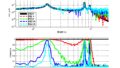
The compliance (frequency response function of displacement/force) of a multi-degree-of-freedom system is Eq. (3.116). near the resonant frequency of the rth order, this rth order vibration mode is the dominant vibration component. Therefore, this resonance peak (around the peak resonance frequency) can be regarded as an approximate one-degree-of-freedom system. For example, in the case of compliance as shown in the figure below, each resonance peak can be regarded as a one-degree-of-freedom system.
$$
G(ω)= x_j / F_i e^{jωt} = (\sum_{r=1}^{N} \frac{ φ_{ri} φ_{rj} }{ -m_r ω^2 + j c_r ω + k_r }) (r=1~N) \tag{3.116}
$$
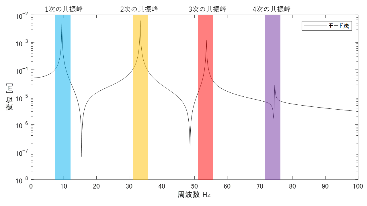
Figure 1: Compliance when resonance peaks are far apart
Note that when the two resonance frequencies are close and the resonance peaks are close to each other, as shown in the figure below, the system cannot be regarded as a one-degree-of-freedom system because of the influence of each other’s vibration components.
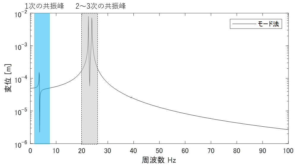 Figure 2 Compliance when resonant peaks are close together
The fact that equation (3.116) can be regarded as one degree of freedom means that ∑ and the subscript r can be omitted, so it can be expressed in equation (6.1).
$$
G(ω) = \frac{ 1/K }{ 1 – β^2 + 2jζβ } , β=\frac{ ω }{Ω} \tag{6.1}
$$
where the magnitude of compliance in equation (6.1) is equation (6.2).
$$
|G(ω)| = \frac{ 1/K }{ \sqrt{ (1 – β^2)^2 + (2ζβ)^2 } } \tag{6.2}
$$
「モード同定」や「モード特性の同定」は測定データ(実験データ)に対して適用します。そのため、この記事のようにn自由度のバネマスモデルで求めた周波数応答関数(コンプライアンスなど)に対してモード同定するのは本来の使い方ではありません。(バネマスモデルであれば、質量行列と剛性行列から共振周波数やモードベクトルなどのモード特性が簡単に求まるので、わざわざ周波数応答関数をモード同定してモード特性を求めるのはナンセンスです。)
ただし、「モード同定」の原理を理解するときにはバネマスモデルを用いた方が、結果の検証などをしやすいのでバネマスモデルを用いて解説をします。
ここからが半値幅法の説明になります。ちなみに半値幅法とは、周波数応答関数からモード減衰比を推定する手法として良く知られていますが、モード減衰比がわかるとモード特性全てを求めることができます。
図1の1次共振峰の拡大図を図3に示します。
“Mode identification” and “Curve-fitting” are applied to measurement data (experimental data). Therefore, mode identification for frequency response functions (compliance, etc.) obtained from an n-degree-of-freedom spring-mass model, as in this article, is not the original usage. (In the case of the spring mass model, it is nonsense to obtain mode characteristics such as resonance frequencies and mode vectors from the mass and stiffness matrices, so it is not necessary to go to the trouble of mode identification of frequency response functions.)
However, when understanding the principle of “mode identification,” it is easier to verify the results by using a spring mass model, so the spring mass model will be used in this explanation.
From here, the half-power method is explained. The half-power method is well known as a method for estimating the modal damping ratio from the frequency response function, but once the modal damping ratio is known, all of the modal characteristics can be obtained.
Figure 3 shows an enlarged view of the first-order resonance peak in Figure 1.
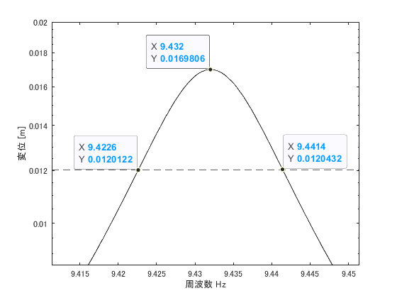 Figure 3 Enlarged view of the first-order resonance peak (m1 self-compliance)
Read the frequencies f1 and f2 at the two points that are 1/√2 of the maximum value|G|max in equation (6.2) (the two points that are -3 dB from the maximum value) and find the mode attenuation ratio ζ from the resonance frequency f0.
$$
ζ= \frac{ f2-f1 }{ 2f_0 } \tag{6.7.1}
$$
Note that the resonance frequency f0 can be obtained without using the resonance frequency f0 using equation (6.7.2).
$$
ζ= \frac{ f2-f1 }{ f2+f1 } \tag{6.7.1}
$$
The maximum value of compliance can also be expressed by Equation (6.5).
$$
|G(ω)|_{max} ≒ \frac{ 1 }{ 2Kζ } \tag{6.5}
$$
Since the amplitude of the mode vector is 1 based on the case where this compliance G(ω) is self-compliant, K in Eq. (6.5) can be treated as equivalent to the modal stiffness k. Self-compliance is, for example, the transfer function obtained from the response of m1 when m1 is vibrated.
Once the modal stiffness k is obtained, the modal mass can be easily obtained from the following equation.
$$
Ω^2 m = k
$$
So far, we know the resonant frequency (the frequency of the maximum peak value, so we know it immediately), the modal damping ratio ζ, the modal stiffness k, and the modal mass m. All that remains is to find the mode vector, and then we will have obtained all the modal characteristics.
In the case of self-compliance, the component of the mode vector is now 1.
For example, in the case of Figure 3, the component of the mode vector corresponding to m1 is 1 at the resonance frequency of 9.432 Hz.
Then how do m2, m3, and …. are obtained?
It is obtained by measuring the mutual compliance Gis (the excitation point is i and the response point is s). φi=1, so the component φs of the mode vector becomes equation (6.11).
$$
K_{is}= \frac{ k }{ φ_s } \tag{6.11}
$$
The relationship to the maximum value of mutual compliance is equation (6.12).
$$
|G_{is}(ω)|_{max} ≒ \frac{ 1 }{ 2K_{is}ζ } \tag{6.12}
$$
Therefore, the component φs of the mode vector can be obtained using equation (6.13).
$$
φ_s ≒ 2kζ|G_{is}(ω)|_{max} \tag{6.13}
$$
Example
Now let us solve Figure 3 as an example.
Answer(theoretical value)
The example problem in Figure 3 is a 4-DOF spring-mass model with the following modal characteristics
First-order resonance frequency: 9.43205759496419 Hz
Modal damping ratio: 0.1%
Modal mass: 1
Modal stiffness: 3512.14651375420
Mode vector:
v=[-0.345365005476218
-0.487723195715426
-0.554079400516416
-0.579521453681323];
Note that the mode vector, mode mass and mode stiffness values will change from the “answer” set here because the half-width method normalizes the excitation point of the mode vector as 1.
So, let’s vibrate m1 and make sure that the component of the mode vector of m1 is 1.
Modal damping ratio: 0.1%
Modal mass: 8.38384691873869
Modal stiffness: 29445.2987274969
Mode vector:
v=[1
1.41219633715614
1.60432988788892
1.67799703065524];
Value obtained by the half-power method
Resonance frequency f0: 9.4320Hz
Frequency at which the maximum value becomes 1/√2 at f1: 9.4226Hz
Frequency at which the maximum value becomes 1/√2 at f2: 9.4414Hz
From equation (6.7.1), the modal damping ratio ζ is about 0.1%.
f0=9.4320;
f1=9.4226;
f2=9.4414;
zeta_hanchi=(f2 - f1)/(f0*2)
zeta_hanchi =

   9.9661e-04
From equation (6.5), we obtain the modal stiffness k and the modal mass m.
Modal stiffness: 29545.6919999358
Modal mass: 8.41253424855546
From equation (6.13), let us find the mode vector.
phys =

    1.0000
    1.4122
    1.6043
    1.6780
We can see that we have correctly identified the mode characteristics.
Cautions for using the half-width method with experimental data
In this article, the frequency response function is obtained in MATLAB, so the frequency resolution can be fine. However, please note that it may not be possible to achieve fine resolution when using experimental data. If the frequency resolution is not fine enough, the frequency at half value is not known and the half-width method cannot be applied.
If you want to obtain a finer frequency resolution with experimental data, measure longer time history data and increase the number of FFT points (number of lines). If impulse excitation was performed and time history data was measured for only about 1 s, the frequency resolution can be increased by adding pseudo-silence (data with zero amplitude).
MATLAB code(Example)
Executable code
Try other cases by changing the frequency resolution of the calculated frequency (freq) and the modal damping ratio (modal_dampimg).
clear all;clc;close all

freq=9.43-0.1:0.0001:9.43+0.1; %計算周波数の定義
w=2*pi*freq; %角振動数

m_vec=ones(1,4);
k_vec=(1:4)*2*10^4;
[M]=eval_Mmatrix(m_vec); %質量行列
[K]=eval_Kmatrix(k_vec); %剛性行列

[V,D]=eig(K,M); %固有値D、固有ベクトルV
for ii1=1:length(m_vec)
    V(:,ii1)=V(:,ii1)/V(1,ii1); % 加振点m1のモードベクトルの成分が1になるように正規化
end
wn=sqrt(diag(D)); %固有角振動数
fn=wn/(2*pi); %固有振動数

mr=diag(V.'*M*V); %モード質量行列
kr=diag(V.'*K*V); %モード剛性行列
c_cr=2*sqrt(mr.*kr);
modal_dampimg=0.1*0.01; %モード減衰比(とりあえず0.1%と設定)
cr=c_cr*modal_dampimg; %モード減衰係数

F=zeros(length(m_vec),1); F(1)=1; %外力ベクトル(全周波数帯を1で加振する)
Xj=zeros(length(m_vec),length(freq)); %変位ベクトル(計算前にベクトルを定義してメモリを確保)

% % % % モード法
ii=1; %加振点 (加振点が複数ある場合はfor ii=1:kength(F)のループを追加すればよい )
for ii1=1:length(m_vec) %応答点
    for ii2=1:length(wn)
        Xj(ii1,:)=Xj(ii1,:)+V(ii1,ii2)*V(ii,ii2)./( -mr(ii2).*w.^2 + 1i*cr(ii2)*w +kr(ii2) )*F(ii);
%       横ベクトル =横ベクトル  +  スカラー  ×スカラー   ./( スカラー×横ベクトル + スカラー×横ベクトル +スカラー)×スカラー
    end
end


figure
semilogy(freq,abs(Xj(1,:)),'k')
hold on
legend('モード法')
xlabel('周波数 Hz')
ylabel('変位 [m]')

figure
semilogy(freq,abs(Xj(1,:)),'k')
hold on
% legend('モード法')
xlabel('周波数 Hz')
ylabel('変位 [m]')
xlim([freq(1) freq(end)])
semilogy([8.5 10],[1 1]*max(abs(Xj(1,:)))/sqrt(2),'--k')

% % % % 半値幅法
f0=9.4320;
f1=9.4226;
f2=9.4414;
zeta_hanchi=(f2 - f1)/(f0*2);
Gmax=max(abs(Xj(1,:)));
k_hanchi=1/(2*zeta_hanchi*Gmax);
m_hanchi=k_hanchi/(2*pi*f0)^2;

% Gis=max(abs(Xj(:,:)),[],2);
% phys=2*k_hanchi*zeta_hanchi*Gis
[Gis,id]=max( abs( imag(Xj(:,:)) ) ,[],2 );
Gis=Gis .* imag(-Xj(:,id(1)))./abs(Xj(:,id(1))) ;
phys=2*k_hanchi*zeta_hanchi*Gis;
function ffile
function [M]=eval_Mmatrix(m_vec)

M=diag(m_vec);

end
function [K]=eval_Kmatrix(k_vec)

K=zeros(length(k_vec));
for ii1=1:length(k_vec)
    if ii1==1
        K(ii1,ii1)=k_vec(ii1);
    else
        K(ii1-1:ii1,ii1-1:ii1)=K(ii1-1:ii1,ii1-1:ii1)+[1 -1;-1 1]*k_vec(ii1);
    end
end

end
コメント