
Introduction
I am re-reviewing the bible-like book “Introduction to Modal Analysis,” which every Japanese vibration engineer has read at least once.
I would like to explain what I have learned in the re-review, showing the MATLAB code. This time, we will review from section 6.2.4, “Curve-fit,” p. 349.
The following link is a summary to a description of vibration theory in English, if you are interested.

I’ve also developed my own curve fitting software.
If you’re interested, feel free to download it from the link below and give it a try.
👉 Free Download
6.2.4 Curve-fit (Curve-fitting)
First, consider the FRF shown in the figure below as an example.

Figure 1 FRF
The Nyquist diagram for the frequency band in the red box shown in Figure 1 is shown in Figure 2.

Figure 2 Nyquist diagram(5~15Hz)
As shown in Figure 2, the Nyquist diagram for FRF is the red line. Depending on the frequency resolution, the Nyquist diagram will be a crisp circle. (However, in textbooks, it is explained as a beautiful circle like the black dotted line…)
モード円適合では、図2に示すようなナイキスト線からモード特性(共振周波数およびモード減衰、モードベクトル)を同定すること意味します。なお、図1および図2は1次共振周波数の共振峰が他の共振周波数の影響を受けていないと考えられます。このような場合にのみモード円適合は適用可能です。
The curve-fitting means identifying the mode characteristics (resonant frequency and mode damping, mode vector) from the Nyquist line as shown in Figure 2. Note that the resonant peaks at the first-order resonant frequency in Figures 1 and 2 are considered to be unaffected by other resonant frequencies. The curve-fitting is applicable only in such cases.
The Nyquist diagram of a resonant peak unaffected by other vibration modes (resonant frequencies) is a circle as shown in Figure 3.

Figure 3 Nyquist diagram of compliance (when the effects of other vibration modes are negligible)
$$
Center = (R, I – \frac{ 1 }{4Kζ}) \tag{6.21}
$$
This also relates to the following eq.
$$
a=2R, b=2I – \frac{ 1 }{2Kζ}, c=\frac{ I }{2Kζ}-R^2-I^2 \tag{6.25}
$$
$$
Radius of circle=\sqrt{c+\frac{ a^2+b^2}{4}}, 中心=(\frac{ a }{2}, \frac{ b }{2}) \tag{6.27}
$$
where the real part of compliance is x and the imaginary part is y. The coefficients a, b, and c can be expressed in terms of the least-squares relationship in equation (6.30). Note that l (lowercase L) means the number of data.
\[
\left[ \begin{array}{ccc}
∑x_i^2 & ∑x_iy_i & ∑x_i \\
∑x_iy_i & ∑y_i^2 & ∑y_i \\
∑x_i & ∑y_i & l \\
\end{array} \right]
\left[ \begin{array}{c} a \\ b \\ c \end{array} \right]
=\left[ \begin{array}{c} ∑(x_i^3+x_iy_i^2) \\ ∑(x_i^2y_i+y_i^3) \\ ∑(x_i^2+y_i^2) \end{array} \right] \tag{6.30}
\]
Equation (6.30) yields a, b, and c, so that a circle with black dotted lines can be drawn as shown in Figure 2.
However, just being able to draw a clean circle does not mean that the mode characteristics (resonant frequency, mode attenuation ratio, and mode vector) can be obtained.
From here, I would like to show the procedure for obtaining the mode characteristics.

Figure 4 Nyquist diagram of compliance part2
First, we need to find the resonance frequency fn shown in Figure 4.
Generally, it is between 9.4Hz and 9.5Hz, so it is often obtained as (9.4Hz + 9.5Hz)/2 = 9.45Hz. However, this was in the early 1990s when Dr. Nagamatsu gave an introduction to modal analysis, and if numerical operations could be performed easily and with high precision as they are today, we would want to be a little smarter about obtaining this.
So how do we obtain the resonance frequency fn?
Since the center of the circle is known from equation (6.27), we know the position on the circle that the resonance frequency fn takes. However, since the correspondence with the frequency is not known, it is necessary to find the correspondence between the position on the circle and the frequency.
As shown in Figure 4, two frequencies (9.4 Hz and 9.5 Hz) straddling the resonance frequency fn are known, so they can be obtained by linear completion as in the following equation.
$$
fn=\frac{θ_d}{θ_d+θ_e}df + fd
$$
Since the angles are linearly complemented, there will be an error, but since the frequency resolution df when curve fitting is performed is about 2 Hz at most, this error may be acceptable.
The mode attenuation ratio can be obtained by finding the resonance frequency fn.
The method for calculating the mode attenuation ratio is shown below.
$$
βd=\frac{fd}{fn}, βe=\frac{fe}{fn} \tag{B9.2}
$$
$$
ζ=\frac{βe^2-βd^2}{2(βd\tan{\frac{θd}{2}}+βe\tan{\frac{θe}{2}})} \tag{B9.5}
$$
The rest of the process is the same as for the half power method. I would like to explain it again just to be sure.
Since the compliance G(ω) is based on the case of self-compliance and the amplitude of the mode vector is 1, K in Eq. (6.5) can be treated as equivalent to the modal stiffness k. Self-compliance is, for example, the transfer function obtained from the response of m1 when m1 is vibrated.
Once the modal stiffness k is obtained, the modal mass can be easily obtained from the following equation.
$$
Ω^2 m = k
$$
So far, the resonant frequency fn, modal damping ratio ζ, modal stiffness k, and modal mass m are known. All that remains is to determine the mode vector, and then we have obtained all the modal characteristics.
In the case of self-compliance, the component of the mode vector is now 1.
On the other hand, for mutual compliance Gis (excitation point is i and response point is s), the following procedure is used to obtain φi=1, so the component φs of the mode vector becomes equation (6.11).
$$
K_{is}= \frac{ k }{ φ_s } \tag{6.11}
$$
The relationship with the value of the resonant frequency of mutual compliance is equation (6.12).
$$
|G_{is}(ωn)| ≒ \frac{ 1 }{ 2K_{is}ζ } \tag{6.12}
$$
Therefore, the component φs of the mode vector can be obtained using equation (6.13).
$$
φ_s ≒ 2kζ|G_{is}(ωn)| \tag{6.13}
$$
Program Verification
We would like to verify the accuracy of the program with the 4dof model. Table 1 shows the theoretical values. We will verify whether these theoretical values can be obtained by the theory of “mode circle fitting. Note that we would also like to verify the relationship with the frequency resolution, since it is known that the accuracy increases with a smaller frequency resolution df.
理論値
| 1st:9.432Hz | 2nd:33.385Hz | 3rd:53.603Hz | 4th:74.490Hz | |
| modal damping ratio:1% | modal damping ratio:1% | modal damping ratio:1% | modal damping ratio:1% | |
| Mode vector | 1 | 1 | 1 | 1 |
| 1.412 | 0.400 | -1.336 | -3.976 | |
| 1.604 | -0.293 | -0.368 | 7.223 | |
| 1.678 | -0.652 | 0.880 | -4.156 |
同定結果(周波数分解能が0.1Hzのとき)
| 1st:9.4727Hz | 2nd:33.4549Hz | 3rd:53.6579Hz | 4th:74.6738Hz | |
| modal damping ratio:1.0057% | modal damping ratio:1.0043% | modal damping ratio:1.0080% | modal damping ratio:1.2731% | |
| Mode vector | 1.0000 | 1.0000 | 1.0000 | 1.0000 |
| 1.3985 | 0.4003 | -1.3234 | -1.9105 | |
| 1.5653 | -0.2944 | -0.3656 | 3.3689 | |
| 1.6323 | -0.6501 | 0.8706 | -1.3685 |
同定結果(周波数分解能が1Hzのとき)
| 1st:9.7776Hz | 2nd:33.9207Hz | 3rd:53.9864Hz | 4th:73.7188Hz | |
| modal damping ratio:1.0772% | modal damping ratio:1.0538% | modal damping ratio:1.0873% | modal damping ratio:1.8900% | |
| Mode vector | 1.0000 | 1.0000 | 1.0000 | 1.0000 |
| 1.2654 | 0.4084 | -1.2482 | -1.2167 | |
| 1.2422 | -0.3108 | -0.3410 | 1.9921 | |
| 1.2617 | -0.6383 | 0.8257 | -1.1708 |
同定結果(周波数分解能が2Hzのとき)
| 1st:10.2043Hz | 2nd:34.5581Hz | 3rd:54.9777Hz | 4th:73.7797Hz | |
| modal damping ratio:1.0647% | modal damping ratio:0.6913% | modal damping ratio:0.9051% | modal damping ratio:18.944% | |
| Mode vector | 1.0000 | 1.0000 | 1.0000 | 1.0000 |
| 1.1764 | 0.2204 | -1.1183 | -0.0953 | |
| 1.2551 | -0.1800 | -0.5794 | 0.1352 | |
| 1.2843 | -0.3242 | 1.4505 | -0.0416 |
Accuracy Comparison
First, the accuracy of the resonant frequency estimation is compared in Table 1. As shown in Table 1, the error is calculated using the theoretical value as the reference (correct value). As can be seen, the smaller the frequency resolution, the smaller the error. Personally, I was surprised that the maximum error is 8.2% when the frequency resolution is 2 Hz. I had expected it to be much lower, so it shows that the frequency resolution setting is important.
Table 1 Resonance frequency estimation accuracy
| 1st resonance freq. Error between theoretical and estimated values [%] | 2nd resonance freq. Error [%] | 3rd resonance freq. Error [%] | 4th resonance freq. Error [%] | |
| df=0.1Hz | 0.4 | 0.2 | 0.1 | 0.2 |
| df=1Hz | 3.7 | 1.6 | 0.7 | 1.0 |
| df=2Hz | 8.2 | 3.5 | 2.6 | 1.0 |
Table 2 then compares the estimation accuracy of the mode attenuation ratios. As shown in Table 2, the larger the frequency resolution, the larger the error and the lower the estimation accuracy. My personal feeling is that a mode attenuation ratio of 60-70% error is acceptable. (In the worst case scenario, it is acceptable if the mode attenuation ratio differs by a factor of 2 or more.)
Therefore, the estimation accuracy of the mode damping ratio for 4th order resonance with a frequency resolution of 2Hz has an unacceptable level of error.
Table 2 Accuracy of Mode Damping Ratio Estimation
| 1st resonance freq. Error between theoretical and estimated values [%] | 2nd resonance freq. Error [%] | 3rd resonance freq. Error [%] | 4th resonance freq. Error [%] | |
| df=0.1Hz | 0.6 | 0.4 | 0.8 | 27.3 |
| df=1Hz | 7.7 | 5.4 | 8.7 | 89.0 |
| df=2Hz | 6.5 | 30.9 | 9.5 | 1794.4 |
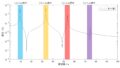
Finally, the accuracy of the mode vector is verified. The accuracy of the mode vector was verified by determining the cross MAC as shown in Figure 5. Although the letters in the figure are smaller, from left to right, the frequency resolution is 0.1 Hz, the center is 1 Hz, and the right is 2 Hz. It can be seen that the mode vector can be obtained with sufficient accuracy at a frequency resolution of 1Hz. At a frequency resolution of 2 Hz, the similarity of (4th order of theory) x (2nd order of mode circle fit) is 0.5, indicating that the mode vector is not well identified.

Figure 5 Accuracy verification results of mode vectors by cross MAC
MATLAB code
Executable program
clear all;clc;close all


m_vec=ones(1,4);
k_vec=(1:4)*2*10^4;
[M]=eval_Mmatrix(m_vec); %mass matrix
[K]=eval_Kmatrix(k_vec); %

[V,D]=eig(K,M); %固有値D、固有ベクトルV
for ii1=1:length(m_vec)
    V(:,ii1)=V(:,ii1)/V(1,ii1); % 加振点m1のモードベクトルの成分が1になるように正規化
end
wn=sqrt(diag(D)); %固有角振動数
fn=wn/(2*pi); %固有振動数

for ii10=1:4
freq=fn(ii10)-7:2:fn(ii10)+7; %計算周波数の定義
w=2*pi*freq; %角振動数


mr=diag(V.'*M*V); %モード質量行列
kr=diag(V.'*K*V); %モード剛性行列
c_cr=2*sqrt(mr.*kr);
modal_dampimg=1*0.01; %モード減衰比(とりあえず0.1%と設定)
cr=c_cr*modal_dampimg; %モード減衰係数

F=zeros(length(m_vec),1); F(1)=1; %外力ベクトル(全周波数帯を1で加振する)
Xj=zeros(length(m_vec),length(freq)); %変位ベクトル(計算前にベクトルを定義してメモリを確保)

% % % % モード法
ii=1; %加振点 (加振点が複数ある場合はfor ii=1:kength(F)のループを追加すればよい )
for ii1=1:length(m_vec) %応答点
    for ii2=1:length(wn)
        Xj(ii1,:)=Xj(ii1,:)+V(ii1,ii2)*V(ii,ii2)./( -mr(ii2).*w.^2 + 1i*cr(ii2)*w +kr(ii2) )*F(ii);
%       横ベクトル =横ベクトル  +  スカラー  ×スカラー   ./( スカラー×横ベクトル + スカラー×横ベクトル +スカラー)×スカラー
    end
end

figure
semilogy(freq,abs(Xj))


% % % % % % % % ここからが「モード円適合」のプログラム
[zeta1,R1,I1,k1,m1,modal_vector1,fn_curve1] = modal_circle_fit(Xj(1,:),freq,[1 1]);
[zeta2,R2,I2,k2,m2,modal_vector2,fn_curve2] = modal_circle_fit(Xj(2,:),freq,[2 1],k1,m1);
[zeta3,R3,I3,k3,m3,modal_vector3,fn_curve3] = modal_circle_fit(Xj(3,:),freq,[3 1],k1,m1);
[zeta4,R4,I4,k4,m4,modal_vector4,fn_curve4] = modal_circle_fit(Xj(4,:),freq,[4 1],k1,m1);

ii10

modal_vector=[
modal_vector1
modal_vector2
modal_vector3
modal_vector4
]

zeta_temp=[
zeta1
zeta2
zeta3
zeta4
];

fn_curve_temp=[fn_curve1
    fn_curve2
    fn_curve3
    fn_curve4];

zeta=mean(zeta_temp);
fn_curve=mean(fn_curve_temp)
zeta*100

end
functionファイル
function [zeta,R,I,k,m,modal_vector,fn_curve]=modal_circle_fit(Xj,freq,out_in,modalk,modalm)
% % Xj コンプライアンス
% % out_in 入力と応答のid、例えば1点応答-2番入力の場合はout_in=[1,2]
df=freq(2) - freq(1);

xi = real(Xj(1,:));
yi = imag(Xj(1,:));

if nargin < 4
    modalk=0;
    modalm=0;
end


A = [sum(xi.^2) sum(xi.*yi) sum(xi)
    sum(xi.*yi) sum(yi.^2) sum(yi)
    sum(xi) sum(yi) length(xi)
    ]; %式(6.30)

B = [sum(xi.^3+xi.*yi.^2)
    sum(xi.^2.*yi+yi.^3)
    sum(xi.^2+yi.^2)
    ]; %式(6.30)

abc=A\B; %式(6.30)

figure
plot(real(Xj(1,:)),imag(Xj(1,:)))
hold on
grid on
axis equal
title([num2str(freq(1)) '~' num2str(freq(end)) 'Hzまで'])


plot(abc(1)/2,abc(2)/2,'ko') %式(6.27)

r=sqrt(abc(3) + (abc(1)^2+abc(2)^2)/4); %式(6.27)
for ii1=0:0.05:2*pi
    plot(abc(1)/2+r*cos(ii1),abc(2)/2+r*sin(ii1),'k.') %式(6.27)
end

% % % % モード円適合で算出された共振周波数の「円上の角度」
fn_theta=atan( abc(2)/abc(1) ); %「円上の角度」≒ 共振周波数
if ( abc(2)/2+r*sin(fn_theta) )^2 < ( abc(2)/2+r*sin(-fn_theta) )^2
    fn_theta=-fn_theta;
end
plot(abc(1)/2+r*cos(fn_theta),abc(2)/2+r*sin(fn_theta),'ko')
Gmax_fn=( abc(1)/2+r*cos(fn_theta) ) + i*( abc(2)/2+r*sin(fn_theta) ); % 「円上の角度」のコンプライアンスの値(共振周波数におけるFRFの値)

% % % % 入力データ|Xj|maxの角度  |G|maxの角度
[value,id_max]=max(abs(Xj(1,:)));
Gmax_theta = atan( imag(Xj(1,id_max))/real(Xj(1,id_max)) );

% % % % 「円上の角度」と隣り合うデータの角度を求める(片方は|G|maxの角度)
if Gmax_theta >= fn_theta
    Gmax_theta_next = atan( imag(Xj(1,id_max+1))/real(Xj(1,id_max+1)) );
    id_next=id_max+1;
else
    Gmax_theta_next = atan( imag(Xj(1,id_max-1))/real(Xj(1,id_max-1)) );
    id_next=id_max-1;
end

% % % % 「円上の角度」と隣り合う角度を求める
dtheta1 = abs( Gmax_theta - fn_theta );
dtheta2 = abs( Gmax_theta - Gmax_theta_next );
% % % % 「円上の角度」から求めた共振周波数(線形補完しているので、共振周波数には誤差があるが、一般的には許容範囲内で収まるはず)
fn_curve=(dtheta1/(dtheta2+dtheta1))*df + freq(id_max);

% % % % atanで角度を求めているので、座標上の第三象限では正負の符号がおかしくなるので、調整する必要がある
if Gmax_theta>0; Gmax_theta = -Gmax_theta; end
if fn_theta>0; fn_theta = -fn_theta; end
if Gmax_theta_next>0; Gmax_theta_next = -Gmax_theta_next; end

theta_d = abs( Gmax_theta - fn_theta );
theta_e = abs( Gmax_theta_next - fn_theta );


beta_d = freq(id_max) / fn_curve; %式(B9.2)
beta_e = freq(id_next) / fn_curve; %式(B9.2)

zeta = abs(beta_e^2 - beta_d^2) / ( 2*(beta_d*tan(theta_d)+beta_e*tan(theta_e)) ); %式(B9.5)

% % % 式(6.25)に代入
R=abc(1)/2;
K=1/(2*zeta)*sqrt( 1/( 4*(abc(3)+R^2) + abc(2)^2) ); % FRFが自己コンプライアンスの場合はk=K;
I=1/2*(abc(2)+1/(2*K*zeta));

% out_in,modalk)
if out_in(1)==out_in(2)
    modal_vector=1;
    k=K;
    m=k/(2*pi*fn_curve)^2;
else
    Gmax_fn
%     Gmax_fn=Gmax_fn .* imag(Gmax_fn)./abs(Gmax_fn)
    modal_vector=2*modalk*zeta*imag(-Gmax_fn);
    k=modalk;
    m=modalm;
end

% [Gis,id]=max(  abs( imag(Xj(:,:)) ) ,[],2  );
% Gis=Gis .* imag(-Xj(:,id(1)))./abs(Xj(:,id(1))) ;
% phys=2*k_hanchi*zeta_hanchi*Gis;
コメント